High school level example 4 (Java Version) : Visualization of the solutions of a f(x)=k equation.

Create a new figure ith the menu item File - New Figure with frame - Without vectors and choose an orthonormal frame.

Create six points of coordinates (-2 ;0), (-1 ;1), (0 ;0), (1 ;-1), (2 ;0) et (4 ;2) (tool ).

Create six calculus named m1, m2, ..., m6 and with formulas respectively 2, 0, -2, 0, 2 et 2 (tool ).

We will now use a predefined construction available with MathGraph32 java (Java version 3.3 or later). This construction allows you to create a function curve going through six points specifying the slope of the tangent lines at these six points.

Use menu item Constructions - Implement predefined construction . A dialog box pops up. Open the directory named Curves through points and slopes and open the construction file named CurveThroughSixPointsWithTangentSlope.

A dialog box pops up for the choice of numerical sources objects. These sources objects are the six tangent slopes.
Assign to the six first elements the calculus m1, m2, m3, m4, m5 and m6, and assign to the element number 7 the frame (O,I,J). Validate by OK.

You must then (as asked for in the indication text area at the bottom of the window) click on the six points created (in increasing order of abscissa). The curve of the function appears.

Pressing key F6 that amonf the final objects is a function named f and coordinates measures of the clicked points.

Activate the blue color and the thin dotted line style (at the top right of the window).

Create now a point linked to the y-axis (tool ) and name this point k (icon ).

Measure the ordinate of point k in (O,I,J) frame (tool . This ordinate is represented as yCoord(k,O,I,J).

Create a new calculus named k with formula yCoord(k,O,I,J) (tool , use button Values).

Create the parallel line to the x-axis through point k (icon ).

Let’s now create a function named g defined by g(t)=f(t)-k (tool with check box Draw Curve not selected).

If necessary, move point k to a position where its ordinate is in the range from 0 to 1.

Use now menu item Calculus -New real calculus - Approximated f(x)=0 root and fill in the dialog box as show below.

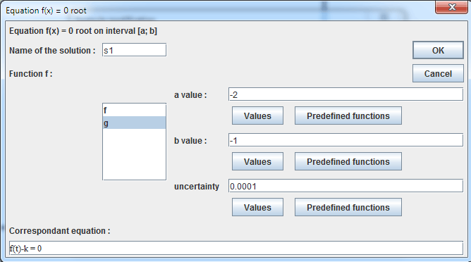
Press F9 key to reactivate last tool and fill in the dialog box as below :

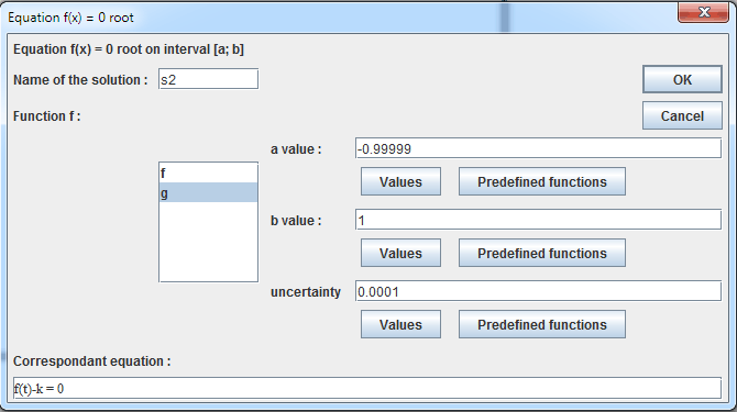
In the same way press F9 and fill in the dialog box :

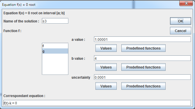
Create now 3 calculus named ys1, ys2 and ys3 with formulas f(s1), f(s2) and f(s3) (tool).

Let’s now visualize the solutions (if existing).

Activate the red color in the color palette.

Create points of coordinates (s1 ; 0), (s2, ;0) and (s3 ; 0) (icon ).

Let’s now create a display of the value of s1 linked to point of coordinates (s1 ;0) with tool . Click on the point and fill in the dialog box as shown below :

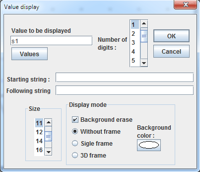
In the same way create a display of the value of s2 linked to the point of coordinates (s2 ;0) and a display of s3 linked to the point of coordinates (s3 ;0).

We want now to calculate and display the number of solutions of the equation f(x)=k.

For this we will create four existence tests.

Use menu itemCalculus >> New real calculus >> Test of value existence. Fill in the dialog box as shown below :

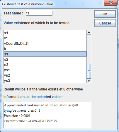
The test t1 value will be 1 when s1 exists and 0 otherwise.

In the same way, create two other existence tests of s2 and s3named t2 and t3.

Create now a calculus named N as shown underneath (tool ).

Calculus N now contains the number of solutions of the equation f(x)=k.

Let’s now use an advanced feature of MathGraph32 : dynamic value insertion in a text display.

First click on tool . Click on the top left part of the figure.

Enter the first part of the text as shown underneath :

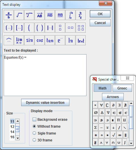
Click on button Dynamic value insertion.

Fill in the new dialog box :

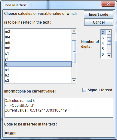
Complete the text field as shown :

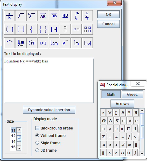
On more time click on button Dynamic value insertion and fill in the new dialog box :

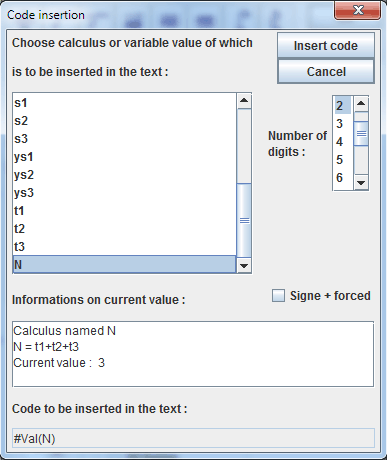
Complete the text editor and validate :

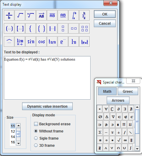
Now capture point k to visualize the solutions of f(x)=k equation and the number of solutions.

Here is the figure animated by MathGraph32 JavaScript motor :

Capture k point.