Linear and exponential regression : Create your own constructionscro constructions

To test this article, you must use version 7.0.0 or more recent of MathGraph32 JS.

Version 7.0 of MathGgraph32 already allows you to create a line of linear regression with tool  : you only have to click on points then on red button STOP to get the line of linear regression of y in x.

But having a macro construction providing the elements of linear regression can be used, for instance, in non linear regressions.

Moreover, this will be an excellent example to learn about macro constructions and matricial calculations.

If your only purpose is to use these macro-constructions, they are available for download at the end of this article.

They both work in the same way : they need a matrix of two columns containing the coordinates of points (x-coordinates in the first column) and the macro construction creates the elements necessary for getting the regression. Then you can use theses elements or graph the regression.

Create a new figure, for instance with a frame.

We will create a matrix of coordinates with very simple values. So we will be able to verify our formulas if necessary.

Use icon at the right side of the calculations toolbar and choose item Matrice.

Fill in the dialog box as underneath..

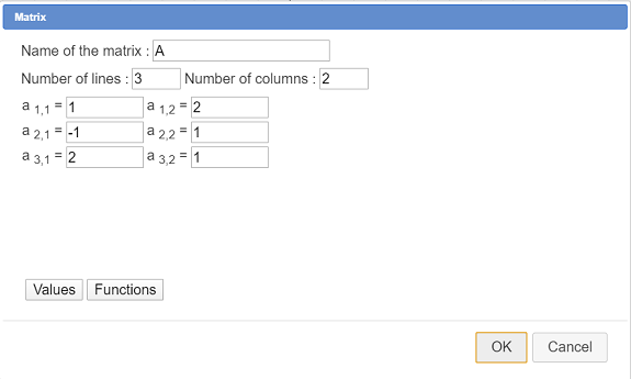
The first column if matrix A contains the x-coordinates and the second one the y-coordinates.

In our calculations we won’t use the real number of lines (here 3à of matrix A because this matrix will be replaced by another when the macro construction will be implemented.

With tool reate the following real calculation :

Calculation name	Formula	Explanations
N	nbrow(A)	In a real calculation, it is the only formula usable for getting the number of lines of a matrix. For instance, 2*nbrow(A) or nbrow(A+1) would not be accepted.

In the following calculations, we will use sum predefined function which operates in this way :

sum(expr, j, start, end, step) : returns sum of expr for j integer getting start value to end with step increment

The 3 last parameters must be integers with start ≤ end and step ≥ 1 (value 1 for step most of the time).

So create the following calculations :

Calculation name	Formula	Explanations
mx	sum(A(k,1),k,1,N,1)/N	will return the x-coordinates mean $\overline{x}$. So we use the first column of matrix A.
my	sum(A(k,2),k,1,N,1)/N	will return the y-coordinates mean $\overline{y}$. So we use the second column of matrix A.
vx	sum(A(k,1)^2,k,1,N,1)/N-mx^2	Will return the x variance according to the formula $\overline{x^2}-(\overline{x})^2$
vy	sum(A(k,2)^2,k,1,N,1)/N-my^2	Will return the y variance according to the formula $\overline{y^2}-(\overline{y})^2$
covxy	sum(A(k,1)*A(k,2),k,1,N,1)/N-mx*my	Will retunr the covariance according to formula $\overline{xy}-\overline{x}\times\overline{y}$
coefcor	covxy/(sqrt(vx)*sqrt(vy))	Wull return the coefficient of linear correlation, in the range 0 to 1. The nearest to 1 the best is the linear approximation.
areg	covxy/vx	Line slope of the regression line
breg	my-areg*mx	Ordinate origin of the regression line going through point $(\overline{x},\overline{y})$

At this stage, you can save your figure. This figure is ready for the creation of our macro construction.

In the upper toolbar, click on icon which make available more tools.

Icon is for the creation of a construction.

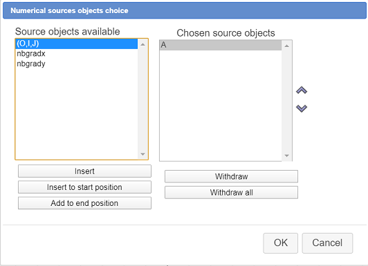
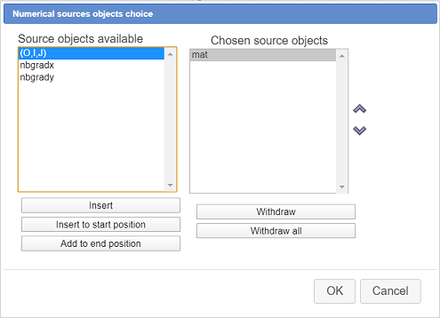
Click on this icon and choose item Numerical sources objects choice.

A dialog box pops up. Click on button Insert (or use double click) to get for only numerical source object matrix A as shown underneath and validate.

Our macro construction will only provide numerical final objects.

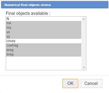
Click again on icon and choose item Numerical final objecst choice.

Select the objects as shown here (you can also select the covariance if you want) :

One more time click on icon and choose item item Finish current construction.

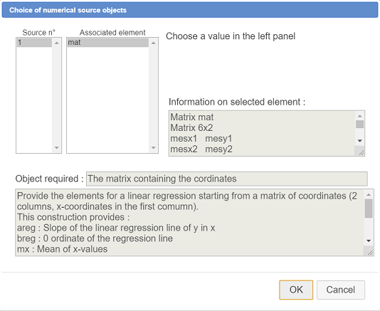
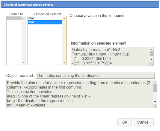
Fill in the dialog box as shown here :

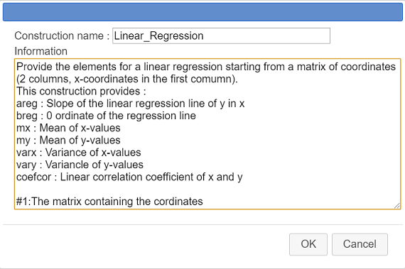
Here is the code to be entered in the information field :

This will give informations to the users of our macro construction.

The last line starting with #1 : provides what will be displayed when the user will implement the consruction when choosing the first (and only) source object (which is a matrix).

We will save our construction in a separate file (with mgc suffix) so as to be able to use it in other figures.

Use icon (macro constructions management) and choose item Save a construction of the figure.

A dialog box pops up. The only construction is already selected. Click on button Save and save your construction in the directory of your choice under the name Linear_Regression.mgc for instance.

Save also your figure in a mgj file. Name it as you want (the macro-construction is part of the figure).

Now we are going to test our construction in a new figure.

With icon , create a new figure with an ortonormal frame.

Use icon (free point) to create 6 free points (you can create more than 6 if you like).

Expand the calculations toolbar, click on icon and choose Matrix of coordinates.

Accept the default name (mat) then click on the 6 points. To finish, click on red button STOP at the bottom right of the window.

For you, MathGraph32 has :

• measured the xand y-coordinates of the 6 points.

• created a matrix with 6 rows and two columns. The first column contains the x-coordinates and the second one the y-coordinates
  • This matrix is dynamic : If you capture one of the free points, the matrix changes.

Now let us include our construction in this new figure and apply it to this matrix.

Use icon (constructions management) and choose item Incorporer une construction depuis un fichier.

Browse to th e directory where you saved your constriction file Linear_Regression.mgc , select it and click on button Open. The construction is now part of your figure.

Use again icon and choose item Implement a construction of the figure.

Our only construction is already selected. Click on button Implement.

A dialog box pops up asking for the sources objects (here only one, a matrix).

Assign matrix mat to the first and only source object as underneath :

In the upper toolbar, use icon to see the numerical objects of the figure.

Activate the red color, a line thickness of 2 pixelsand activate tool (line through equation in a frame).

Assign to the equation line the formula : y=areg*x+breg and validate as underneath :

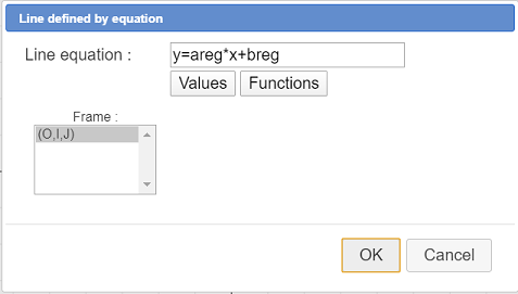
You line of linear regression appears. The more the points are aligned, the more the line is near them.

We now are going to create a new figure allowing us to create a macro construction of exponential regression.

Use icon to create a new figure.

Expanding the calculation toolbar, click on the right on and choose item item Matrix.

Create the matrix mat as shown here :

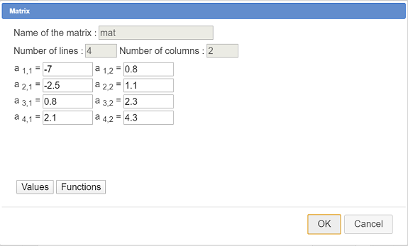
Then use icon to create a real calculation named N with formula nbrow(mat).

First let us recall the bottom line : if the points coordinates of which are contained in matrix mat are "near" an exponential function curve, instead of approaching the points by a line (linear regression) , we will try to approach it by a curve of equation $y=A\times x^{ r}$ (which implies all the y-coordinates are positive).

When y > 0, $y=Ar^x$⇔$\ln (y)=\ln (A)+ \ln (x^r)$⇔$\ln (y)=\ln (A)+ x\ln (r) $.

writing $y’=\ln{y}, \ln(A)=a$ et $\ln(r)=b$ the last equality is of type $y’=ax+b$

The idea is so to create a two column matrix. Ths first column of this new matrix will be the same as matrix mat and the second column will containt the logarithm of the second column of matrix mat.

Then we will apply to this new matrix our construction of linear regression which will provide us the values of areg and breg.

We will then infer $A=e^{areg}$ and $r=e^{breg}$

So let us create this new matrix.

Expanding the calculations toolbar, use at the right icon and choose item Matrix by formula.

Fill in the dialog box as shown here :

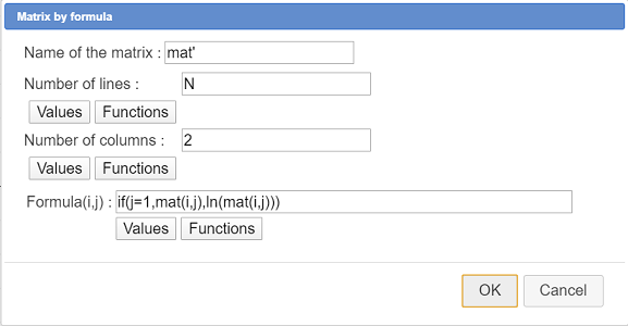
Here is the formula used :

Use icon (constructions management) and choose item Incorporate construction from file.

Browse to the directory you saved your Regression_Lineaire.mgc file to , select the file and click on button Open.

Again use con and choose item Implement a construction of the figure.

Our only construction is already selected. Click on button Implement.

Fill in the dialog box as shown here :

Using icon you can now see the objects added by the construction. Among the calculations areg and breg.

Now use tool to create the following real calculations :

Calculation name	Formula
A	exp(areg)
r	exp(breg)

Now let us create the function approximating y function of x with icon as underneath (don’t check the checkbox Create curve)

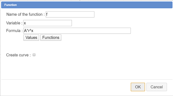
Function name	Formula
f	A*r^x

Our figure is now ready to create our new macro construction of exponential regression.

Activate tool (construction creation) and choose item Numerical sources objects choice.

For only numerical source object choose mat as underneath :

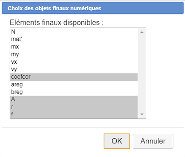
Again activate tool and choose item Numerical final objects choice.

Select coefcor (corelation coefficient), A, r ans f as shown here :

Activate again tool and choose item Finish current construction.

Fill in the dialog box as shown here :

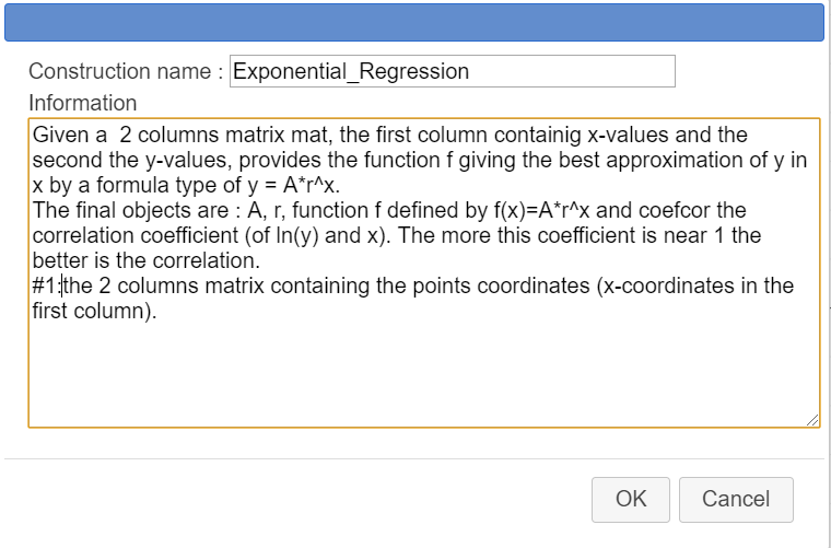
Here is the content of the information field :

Your new construction is now part of your figure.

To save the construction in a mgc file, use icon (constructions management) and choose item Save a construction of the figure. Save it under the name Exponential_Regression.mgc.

It is also better to save the figure iself, in the case you could have made a mistake while creating the macro construction.

Now we are going to test our new construction in another figure.

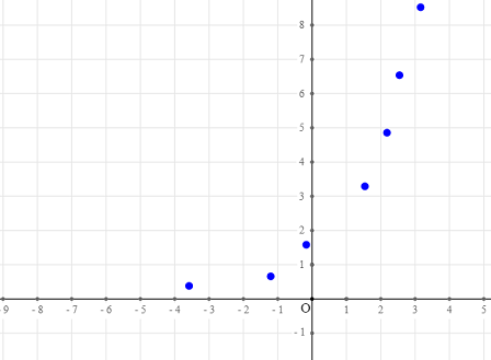
Create a new figure with a frame using icon (upper toolbar) and create a few free points like underneath, so that the points seem to be near an exponential curve..

Now we are going to ask MathGraph to create a matrice coordinates of which will be the coordinates of the free points just created.

Expanding the calculation toolbar, clcik on icon and choose item Matrix of coordinates.

Accept the name mat for the matrix then click on the free points you created before. When you are done clicking on the last point, click on the red button STOPon the bottom right side of the window.

If you use tool you will see that MathGraph32 has measured the x and y coordinates of the points the created a two columns matrix mat containing these measures.

Let us incorporate in this figure our construction of exponential regression.

Use icon and choose item Incorporate construction from file.

Browse to the directory you savec your constrction in, then click on button Open. The construction is now part of your figure.

Again use icon and choose item Implement a construction of the figure. Select the exponential regression consruction and click on button Implement.

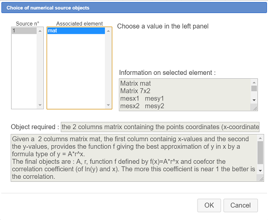
A dialog box pops up for the choice of the sources objects (only one here, a matrix).

Fill in the dialog box as underneath, assigning for the source object the matrix mat and validate.

In the upper toolbar, use icon to see the numerical objects of the figure.

At the bottom of the list, you see the objects created by the construction, coefcor, A, r et function f.

Let us now graph function f.

In the color palette, actiavte the red color then use tool (expanding the locuses toolbar).

Ask for the curve of function f to graph on R.

To finish, let us display the value of the correlation coefficient with the value display tool .

Click at the top left of the figure and fill in the dialog box as underneath :

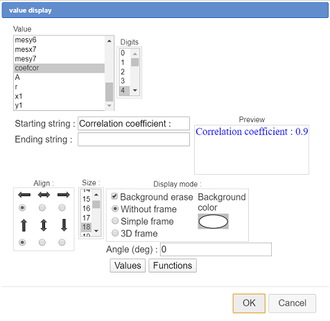
You can now capture the points of the figure. The more the curve is near the points, the more the correlation coefficient is near 1.

Voici ci-dessous la figure finale :

Vous pouvez télécharger ces deux macro constructions dans des fichiers zip ci-dessous :