Logiciel libre de géométrie, d'analyse et de simulation multiplateforme par Yves Biton
Toutes les versions de cet article : [English] [Español] [français]
This example implies a great calculation power but the calculation engine of MathGraph32 is fit.
You can see below this figure in action. Click on macro Animer la roue to lauch the animation.
Start MathGraph32 (JavaScript version) and use icon  to create a new figure with an orthonormal frame.
Use icon  (figure options) and make sure the checkbox radian is checked for the unity angle of the figure.
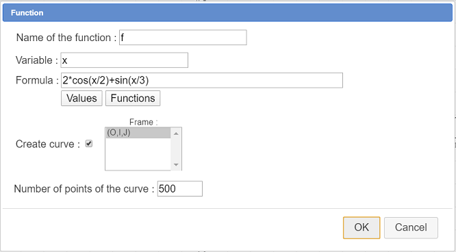
Expanding the calculation toolbar (Third row from the bottom), use now icon  , and create a function f as shown underneath. Let the checkbox Create curve checked.
Now let us ask MathGraph32 to calculate the formal derivative of function f.
For this use icon  . In the dialog box popping up, the function f is already selected. Name this derivative f ’ and validate.
First a preliminary statement : The (algebrical) length of the arc of curve of function f between abscissa 0 and a is given by the formula $ \int_{0}^{a} \sqrt{1+(f’(x))^2}dx $ (with f derivable and the f dérivative continuous).
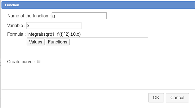
Use icon to create a function g as underneath, unchecking the checkbox Draw Curve (This function will be used to calculate the approximated length of f arcs of curve ).
Here is the formula to be used for g(x) : integrale(sqrt(1+f'(t)^2),t,0,x)
Please remember that a click on the button Functions you are given a list of the predefined functions and the syntax to be used for each function.
Here, the first parameter is the formula to be integrated, the second parameter is the name of the formal variable used in this function (here t), the third parameter i the lower bound of integration et the fourth the upper bound of integration.
So g(x) will represent the algebrical length of the arc of curve of fonction f between abscissa 0 and x.
Now use icon  to create two real calculations like underneath :
| Name of the calculation | Formula | Comments |
| L | g(16) | L will represent the algebrical length of the arc of cuurve of function f between abbscissa 0 and 16. This number is positive |
| L’ | g(-16) | will represent the algebrical length of the arc of cuurve of function f between abbscissa 0 and -16. This number is negative |
Now we are going to create a cursor with values in the range L’ to L.
For this, activate icon  in the calculations toolbar ; click on the upper left corner of the figure.
Fill in the dialog box as shown here :
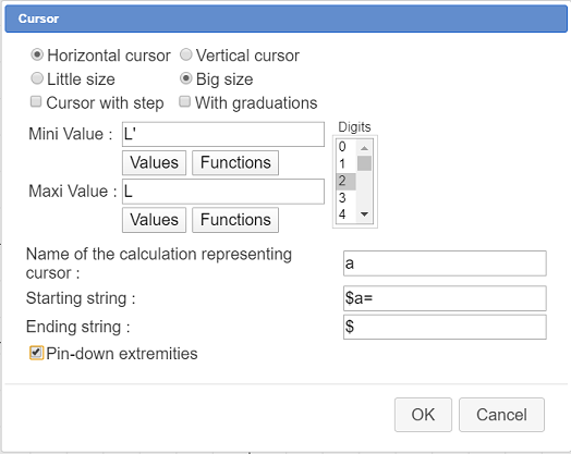
Here we ask for a cursor of big size and with non integer values. The characters $ purpose is to display the starting string in LaTeX mode.
The value of a will represent the algebrical lenth the circle has been running through (starting from abscissa 0)
For each value of a we need to know the abscissa x of the curve for which this length has been run through by the circle.
We will calculate x as an approximate root of an equation.
For this use ico  and fill in the dialog box as shown here :
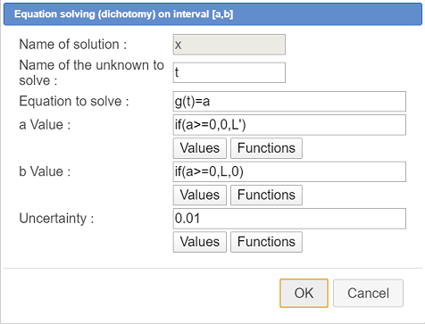
The equation to be solved is g(t)=a (of unknown t) and we ask for the solution of this equation on interval [0 ; L] if a is positive and [L’ ; 0] if a is negative (the calculation of the approximated root is faster if the interval is smaller). That is the reason why we use an if in the formulas for a and b values (lower and upper bound of the interval on which we search for the root x).
The calculation of x uses a lot of system power because each value of x is calculated by dichotomy and, moreover, the function g used to calulate this root uses an integral which is also calculated by approximation.
Now it is time to create the wheel that will roll on the curve.
First let us create a variable r that will represent the radius of the wheel.
Use icon  to create a variable named r with 0.25 as mini value, 1.5 as maxi value, 0.25 for step value et 1 for actual value.
Check the checkbox Associated dialog. Buttons + and - associated to this variable will be available at the right bottom of the figure.
In the color palette, use maroon color.
Use icon  and ask for the point of coordinates (x ; 0).
Expanding the display toolbar, use icon  to create a LaTeX display linked to the last point created (click first on the point then a dialog bow pops up). Enter x as code LaTeX and ask for a display centered horizontaly et under the point. Then you can move this LaTeX with tool
  to get it positionned a little lower.
The creation of this LaTeX dispolay is not mandatory for the rest of the construction..
Use again icon ans ask for the point of coordinates (x ; f(x)). Thus this is the point of the curve with x for abscissa.
Activate the dotted line style and use icon  to create a segment joining the points of coordinates (x ; 0) et (x ; f(x))
Now let us create the tangent to the curve at this last point
For this use icon  (line through slope), click on the last point created and, in the dialog box popping up, enter for slope : f’(x).
Now use tool to create the line perpendicular to this tangent and going through the point of the curve : click first on the tangent then on the point of coordinates (x ;f (x)). This line is the normal to the curve at rhis point.
Use icon  to create the circle with center the point of coordinates (x ; f(x)) and radius r (where r is the variable defined before).
Use tool  to create the intersection of this circle with the normal to the curve (just click at the intersection when this intersection is displayed near the mouse pointer).
Two intersection points appear. We will use only the point that is above the curve. Le t us name it A.
Now let us create the wheel. In the color palette, activate the blue color and choose a continuous line style with a 2 pixels width.
Use tool  to create the circle of center A and going through the point of the curve. This circle will be our "wheel".
Use now tool  of the upper toolbar to mask : the first circle, the second intersection point, the two lines (tangent et normal).
Now we are going to create rays for the "wheel".
In the color palette, activate red color and activate the dotted line style.
Expand the transformation toolbar and use icon  (rotation icon)
First click on the center of the last circle the wheel center). A dialog box pops up asking for the rotation angle.
For angle of the rotation, enter -a/r the validate as here :
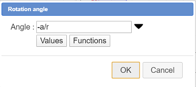
Here we use the formula giving the lenth of a circle arc : $Long = r \times \vartheta$. Here the length of the arc is a. But don’t fotget the minus sign.
Then click on the point of coordinates (x ; f(x)) (point of the curve).
The image point you just just created represent the actual position of the wheel point that was under the wheel when the wheel was at the abscissa 0.
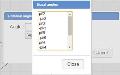
Now use again the rotation icon and click on the center of the wheel. This time choose for angle pi/3 (you can choose one of the predefined angles by clicking on the black arrow lihe underneath).
Click on the point you just created to get it’s image then click again on the new point and proceed 5 times to get six points regularly spaced on the wheel
Then join the opposite points by three segments like this :
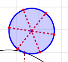
.
You can already see that, when capturing the mobile point of the cursor the "wheel" rolls on the curve.
Now we will create an animation macro to get the wheel roll automatically.
For this expland the displays toolbar and, on the right, click on icon  (like underneath) then choose Animated macro of linked point.

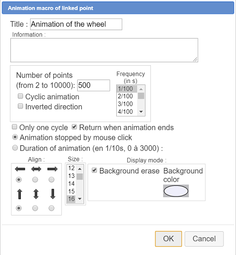
First you are asked to click on the spot the macro is to be displayed at : click under the cursor.
Fill in the dialog box as shown here :
If you want now to launch the animation, in the upper toolbar, click on icon  then click on the macro. Clicl again on the figure to get the animation stop.
On the bottom right corner of the figure you can click on buttond + and - to make the radius of the wheel vary.
Let us give a last improvement to our figure by adding a formula editor allowing the user to modify the formula of f(x) directly on the figure.
Expand the displays toolbar and click on icon  .
.
The click at the spot this editor is to be displayed (for instance at the middle top of the figure) then fill in the dialog box as shown here :
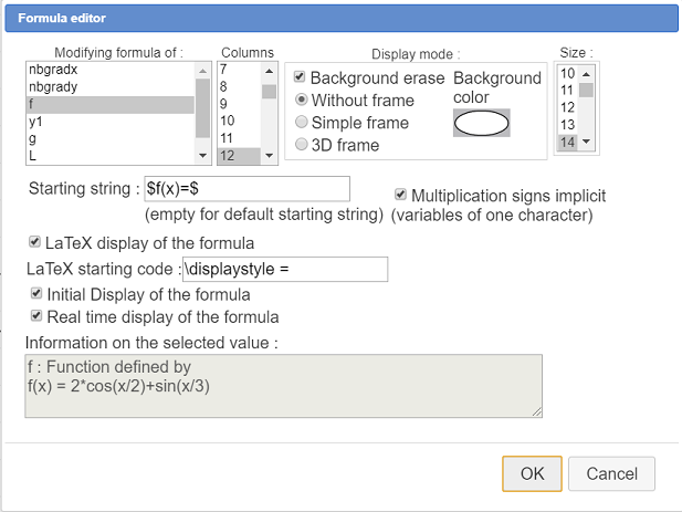
You can now change the formula of function f. Better if the curve is not too irregular !
Here is the Base 64 code of this figure :
TWF0aEdyYXBoSmF2YTEuMAAAABM+TMzNAAJmcv###wEA#wEAAAAAAAAAAAUsAAAC2AAAAQEAAAAAAAAAAAAAAGb#####AAAAAQAKQ0NhbGNDb25zdAD#####AAJwaQAWMy4xNDE1OTI2NTM1ODk3OTMyMzg0Nv####8AAAABAApDQ29uc3RhbnRlQAkh+1RELRj#####AAAAAQAPQ1ZhcmlhYmxlQm9ybmVlAP####8AAXI#8AAAAAAAAD#QAAAAAAAAP#QAAAAAAAA#0AAAAAAAAAEABDAuMjUABDEuMjUABDAuMjX#####AAAAAQAKQ1BvaW50QmFzZQD#####AAAAAAAOAAFPAMAoAAAAAAAAAAAAAAAAAAAAAAUAAUB9QAAAAAAAQHINcKPXCj7#####AAAAAQAUQ0Ryb2l0ZURpcmVjdGlvbkZpeGUA#####wEAAAAAEAAAAQAAAAEAAAACAT#wAAAAAAAA#####wAAAAEAD0NQb2ludExpZURyb2l0ZQD#####AAAAAAEOAAFJAMAYAAAAAAAAAAAAAAAAAAAAAAUAAUA6AAAAAAAAAAAAA#####8AAAABAAlDRHJvaXRlQUIA#####wAAAAAAEAAAAQAAAAEAAAACAAAABP####8AAAABABZDRHJvaXRlUGVycGVuZGljdWxhaXJlAP####8AAAAAABAAAAEAAAABAAAAAgAAAAX#####AAAAAQAJQ0NlcmNsZU9BAP####8BAAAAAAAAAQAAAAIAAAAE#####wAAAAEAEENJbnREcm9pdGVDZXJjbGUA#####wAAAAYAAAAH#####wAAAAEAEENQb2ludExpZUJpcG9pbnQA#####wEAAAAAEAAAAQAABQABAAAACAAAAAoA#####wAAAAABDgABSgDAKAAAAAAAAMAQAAAAAAAAAAAFAAIAAAAI#####wAAAAIAB0NSZXBlcmUA#####wDm5uYAAAABAAAAAgAAAAQAAAAKAQEAAAAAAQAAAAAAAAAAAAAAAQAAAAAAAAAAAAAAAT#wAAAAAAAAAAAAAT#wAAAAAAAA#####wAAAAEACkNVbml0ZXhSZXAA#####wAEdW5pdAAAAAv#####AAAAAQALQ0hvbW90aGV0aWUA#####wAAAAL#####AAAAAQAKQ09wZXJhdGlvbgMAAAABP#AAAAAAAAD#####AAAAAQAPQ1Jlc3VsdGF0VmFsZXVyAAAADP####8AAAABAAtDUG9pbnRJbWFnZQD#####AQAAAAAQAAJXIgEAAAEAAAAABAAAAA3#####AAAAAQAJQ0xvbmd1ZXVyAP####8AAAACAAAADv####8AAAABAAdDQ2FsY3VsAP####8AB25iZ3JhZHgAAjIwAAAAAUA0AAAAAAAAAAAAEgD#####AAduYmdyYWR5AAIyMAAAAAFANAAAAAAAAP####8AAAABABRDSW1wbGVtZW50YXRpb25Qcm90bwD#####ABRHcmFkdWF0aW9uQXhlc1JlcGVyZQAAABsAAAAIAAAAAwAAAAsAAAAQAAAAEf####8AAAABABNDQWJzY2lzc2VPcmlnaW5lUmVwAAAAABIABWFic29yAAAAC#####8AAAABABNDT3Jkb25uZWVPcmlnaW5lUmVwAAAAABIABW9yZG9yAAAACwAAAAwAAAAAEgAGdW5pdGV4AAAAC#####8AAAABAApDVW5pdGV5UmVwAAAAABIABnVuaXRleQAAAAv#####AAAAAQAQQ1BvaW50RGFuc1JlcGVyZQAAAAASAAAAAAAQAAABAAAFAAAAAAsAAAAPAAAAEwAAAA8AAAAUAAAAFwAAAAASAAAAAAAQAAABAAAFAAAAAAsAAAAOAAAAAA8AAAATAAAADwAAABUAAAAPAAAAFAAAABcAAAAAEgAAAAAAEAAAAQAABQAAAAALAAAADwAAABMAAAAOAAAAAA8AAAAUAAAADwAAABYAAAANAAAAABIAAAAXAAAADwAAABAAAAAQAAAAABIAAAAAABAAAAEAAAUAAAAAGAAAABoAAAANAAAAABIAAAAXAAAADwAAABEAAAAQAAAAABIAAAAAABAAAAEAAAUAAAAAGQAAABz#####AAAAAQAIQ1NlZ21lbnQAAAAAEgEAAAAAEAAAAQAAAAEAAAAYAAAAGwAAABgAAAAAEgEAAAAAEAAAAQAAAAEAAAAZAAAAHQAAAAUAAAAAEgEAAAAACwABVwDAFAAAAAAAAMA0AAAAAAAAAAAFAAE#3FZ4mrzfDgAAAB7#####AAAAAgAIQ01lc3VyZVgAAAAAEgAGeENvb3JkAAAACwAAACAAAAASAAAAABIABWFic3cxAAZ4Q29vcmQAAAAPAAAAIf####8AAAACABJDTGlldU9iamV0UGFyUHRMaWUBAAAAEgBmZmYAAAAAACAAAAAPAAAAEAAAACAAAAACAAAAIAAAACAAAAASAAAAABIABWFic3cyAA0yKmFic29yLWFic3cxAAAADgEAAAAOAgAAAAFAAAAAAAAAAAAAAA8AAAATAAAADwAAACIAAAAXAAAAABIBAAAAABAAAAEAAAUAAAAACwAAAA8AAAAkAAAADwAAABQAAAAaAQAAABIAZmZmAAAAAAAlAAAADwAAABAAAAAgAAAABQAAACAAAAAhAAAAIgAAACQAAAAlAAAABQAAAAASAQAAAAALAAFSAEAgAAAAAAAAwCAAAAAAAAAAAAUAAT#RG06BtOgfAAAAH#####8AAAACAAhDTWVzdXJlWQAAAAASAAZ5Q29vcmQAAAALAAAAJwAAABIAAAAAEgAFb3JkcjEABnlDb29yZAAAAA8AAAAoAAAAGgEAAAASAGZmZgAAAAAAJwAAAA8AAAARAAAAJwAAAAIAAAAnAAAAJwAAABIAAAAAEgAFb3JkcjIADTIqb3Jkb3Itb3JkcjEAAAAOAQAAAA4CAAAAAUAAAAAAAAAAAAAADwAAABQAAAAPAAAAKQAAABcAAAAAEgEAAAAAEAAAAQAABQAAAAALAAAADwAAABMAAAAPAAAAKwAAABoBAAAAEgBmZmYAAAAAACwAAAAPAAAAEQAAACcAAAAFAAAAJwAAACgAAAApAAAAKwAAACz#####AAAAAgAMQ0NvbW1lbnRhaXJlAAAAABIBZmZmAAAAAAAAAAAAQBgAAAAAAAAAAAAAACALAAH###8AAAABAAAAAAAAAAEAAAAAAAAAAAALI1ZhbChhYnN3MSkAAAAaAQAAABIAZmZmAAAAAAAuAAAADwAAABAAAAAgAAAABAAAACAAAAAhAAAAIgAAAC4AAAAcAAAAABIBZmZmAAAAAAAAAAAAQBgAAAAAAAAAAAAAACULAAH###8AAAABAAAAAAAAAAEAAAAAAAAAAAALI1ZhbChhYnN3MikAAAAaAQAAABIAZmZmAAAAAAAwAAAADwAAABAAAAAgAAAABgAAACAAAAAhAAAAIgAAACQAAAAlAAAAMAAAABwAAAAAEgFmZmYAwCAAAAAAAAA#8AAAAAAAAAAAAAAAJwsAAf###wAAAAIAAAABAAAAAQAAAAAAAAAAAAsjVmFsKG9yZHIxKQAAABoBAAAAEgBmZmYAAAAAADIAAAAPAAAAEQAAACcAAAAEAAAAJwAAACgAAAApAAAAMgAAABwAAAAAEgFmZmYAwBwAAAAAAAAAAAAAAAAAAAAAAAAALAsAAf###wAAAAIAAAABAAAAAQAAAAAAAAAAAAsjVmFsKG9yZHIyKQAAABoBAAAAEgBmZmYAAAAAADQAAAAPAAAAEQAAACcAAAAGAAAAJwAAACgAAAApAAAAKwAAACwAAAA0#####wAAAAEABUNGb25jAP####8AAWYAEzIqY29zKHgvMikrc2luKHgvMykAAAAOAAAAAA4CAAAAAUAAAAAAAAAA#####wAAAAIACUNGb25jdGlvbgQAAAAOA#####8AAAACABFDVmFyaWFibGVGb3JtZWxsZQAAAAAAAAABQAAAAAAAAAAAAAAeAwAAAA4DAAAAHwAAAAAAAAABQAgAAAAAAAAAAXgAAAAFAP####8BAAAAABAAAXgAAAAAAAAAAABACAAAAAAAAAAABQABv#5GMaUabogAAAAFAAAAGQD#####AAJ4MQAAAAsAAAA3AAAAEgD#####AAJ5MQAFZih4MSn#####AAAAAQAOQ0FwcGVsRm9uY3Rpb24AAAA2AAAADwAAADgAAAAXAP####8BAAAAABAAAAAAAAAAAAAAAEAIAAAAAAAAAAAFAAAAAAsAAAAPAAAAOAAAAA8AAAA5#####wAAAAIADUNMaWV1RGVQb2ludHMA#####wAAAAAAAAABAAAAOgAAAfQAAQAAADcAAAAEAAAANwAAADgAAAA5AAAAOv####8AAAABAAhDRGVyaXZlZQD#####AAJmJwAAADYAAAAdAP####8AAWcAIGludGVncmFsZShzcXJ0KDErZicodCleMiksdCwwLHgp#####wAAAAEAFUNJbnRlZ3JhbGVEYW5zRm9ybXVsZQABdAAAAB4BAAAADgAAAAABP#AAAAAAAAD#####AAAAAQAKQ1B1aXNzYW5jZQAAACAAAAA8AAAAHwAAAAEAAAABQAAAAAAAAAAAAAABAAAAAAAAAAAAAAAfAAAAAAABeAAAABIA#####wABTAAFZygxNikAAAAgAAAAPQAAAAFAMAAAAAAAAAAAABIA#####wACTCcABmcoLTE2KQAAACAAAAA9#####wAAAAEADENNb2luc1VuYWlyZQAAAAFAMAAAAAAAAAAAAAMA#####wAAAAAAEAAAAEAIAAAAAAAAAAAAAAAAAAAAAAUAAEBFgAAAAAAAQD#XCj1wo9gAAAATAP####8AB0N1cnNldXIAAAAFAAAABQAAAAMAAAA#AAAAPgAAAEAAAAAEAAAAAEEBAAAAABAAAAEAAAABAAAAQAE#8AAAAAAAAAAAAAUBAAAAQQAAAAAAEAAAAMAIAAAAAAAAP#AAAAAAAAAAAAUAAEBtQAAAAAAAAAAAQgAAAA0AAAAAQQAAAEAAAAAOAwAAAA8AAAA#AAAADgEAAAAPAAAAPwAAAA8AAAA+AAAAEAAAAABBAQAAAAANAAJPMQDAEAAAAAAAAEAQAAAAAAAAAAAFAAAAAEMAAABEAAAADQAAAABBAAAAQAAAAA4DAAAADgEAAAABP#AAAAAAAAAAAAAPAAAAPwAAAA4BAAAADwAAAD4AAAAPAAAAPwAAABAAAAAAQQEAAAAADQACSTEAwAAAAAAAAABACAAAAAAAAAAABQAAAABDAAAARgAAABgBAAAAQQAAAAAAEAAAAQAAAAEAAABAAAAAQwAAAAUBAAAAQQAAAAABEAACazEAwAAAAAAAAABAAAAAAAAAAAAAAQABP+JTJTJTJTIAAABI#####wAAAAIAD0NNZXN1cmVBYnNjaXNzZQEAAABBAAFhAAAARQAAAEcAAABJ#####wAAAAEAD0NWYWxldXJBZmZpY2hlZQEAAABBAAAAAAAAAAAAAAAAAMAYAAAAAAAAAAAAAABJDwAB####AAAAAQAAAAIAAAABAAAAAAAAAAAAAyRhPQABJAIAAABK#####wAAAAIAEUNTb2x1dGlvbkVxdWF0aW9uAP####8AAXgAAXQAAAAOCAAAACAAAAA9AAAAHwAAAAAAAAAPAAAASgAAAA4BAAAAIAAAAD0AAAAfAAAAAAAAAA8AAABK#####wAAAAEADUNGb25jdGlvbjNWYXIAAAAADgcAAAAPAAAASgAAAAEAAAAAAAAAAAAAAAEAAAAAAAAAAAAAAA8AAAA#AAAAKQAAAAAOBwAAAA8AAABKAAAAAQAAAAAAAAAAAAAADwAAAD4AAAABAAAAAAAAAAAAAAABP4R64UeuFHsAAAAXAP####8AfwAAABAAAAAAAAAAAAAAAEAIAAAAAAAAAAAFAAAAAAsAAAAPAAAATAAAAAEAAAAAAAAAAP####8AAAACAAZDTGF0ZXgA#####wB#AAAAv#AAAAAAAABAGAAAAAAAAAAAAAAATRIAAAAAAAEAAAAAAAAAAQAAAAAAAAAAAAF4AAAAFwD#####AH8AAAAQAAAAAAAAAAAAAABACAAAAAAAAAAABQAAAAALAAAADwAAAEwAAAAgAAAANgAAAA8AAABMAAAAGAD#####AH8AAAAQAAABAAABAQAAAE0AAABP#####wAAAAEACUNEcm9pdGVPbQD#####AQAA#wAQAAABAAABAQAAAAsAAABPAAAAIAAAADwAAAAPAAAATAAAAAcA#####wEAAP8AEAAAAQAAAQEAAABPAAAAUf####8AAAACAAlDQ2VyY2xlT1IA#####wEAAP8AAAEBAAAATwAAAA8AAAABAAAAAAkA#####wAAAFIAAABTAAAACgD#####AQAA#wAQAAAAAAAAAAAAAABACAAAAAAAAAAABQABAAAAVAAAAAoA#####wAAAP8AEAAAAAAAAAAAAAAAQAgAAAAAAAAAAAUAAgAAAFQAAAAIAP####8AAAD#AAAAAgAAAFYAAABP#####wAAAAEACUNSb3RhdGlvbgD#####AAAAVgAAACUAAAAOAwAAAA8AAABKAAAADwAAAAEAAAAQAP####8A#wAAABAAAAAAAAAAAAAAAEAIAAAAAAAAAAAFAAAAAE8AAABYAAAALQD#####AAAAVgAAAA4DAAAADwAAAAAAAAABQAgAAAAAAAAAAAAQAP####8A#wAAABAAAAAAAAAAAAAAAEAIAAAAAAAAAAAFAAAAAFkAAABaAAAAEAD#####AP8AAAAQAAAAAAAAAAAAAABACAAAAAAAAAAABQAAAABbAAAAWgAAABAA#####wD#AAAAEAAAAAAAAAAAAAAAQAgAAAAAAAAAAAUAAAAAXAAAAFoAAAAQAP####8A#wAAABAAAAAAAAAAAAAAAEAIAAAAAAAAAAAFAAAAAF0AAABaAAAAEAD#####AP8AAAAQAAAAAAAAAAAAAABACAAAAAAAAAAABQAAAABeAAAAWgAAABgA#####wD#AAAAEAAAAQAAAQIAAABZAAAAXQAAABgA#####wD#AAAAEAAAAQAAAQIAAABbAAAAXgAAABgA#####wD#AAAAEAAAAQAAAQIAAABcAAAAX#####8AAAABAA5DU3VyZmFjZURpc3F1ZQD#####AAAA#wAAAAAABQAAAFf#####AAAAAgAXQ01hY3JvQW5pbWF0aW9uUG9pbnRMaWUA#####wAAAP8BAAD#####EEBFgAAAAAAAQFL1wo9cKPYCAe#v+wAAAAAAAAAAAAAAAQAAAAAAAAAAABFBbmltYXRlIHRoZSB3aGVlbAAAAAAAAAoAAAH0AAAAAAAAAEkAAQD#####AAAABAAPQ0VkaXRldXJGb3JtdWxlAP####8AAAAAAQAA#####w5AdpAAAAAAAEA11wo9cKPYAAH###8AAAACAAAAAAAAAAEAAAAAAAAAAAAAADYAByRmKHgpPSQAAAAMAQEAAT0BAQAAAA###########w== Accueil
 Présentation
 FAQ
FAQ Contact