Visualization of planes in pseudo 3D

We will show here how to use MathGraph32 to visualize planes and other objects in 3D.

This article has been adapted to the JavaScript version of MathGraph32.

Start by creating a 3D figure with an orthonormal frame with icon , choose Basic 3D figure then choose item Orthonormal 3D frame.

Now we will create four cursors that will contain the four parameters of our plan equation $ax+by+cz+d=0$.

Click on icon (cursor creation). Click on the top left corner of the figure and fill in the dialog box as underneath. Here we create a cursor with integer values in the range -6 to 6..

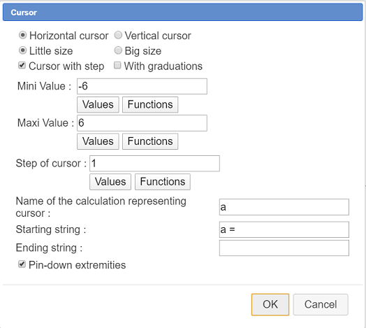
To be noted : The edges of the cursor are point pinned downd by default. If you want to move the cursor or get it bigger you will have first to unpin these points using toll .

In the same way, create three other cursors with integer values (in the range -6 to 6) under the first one for the values of b, c and d.

With JavaScript version of MathGraph32, the predefined macro constructions must be downloaded separatly on MathGraph32 webpage on this page Download of MathGraph32 version 7.9.

So we will assume here that you have dowloaded the last version of the predefined macro constructions on MathGraph32 website and expanded the zip file in a folder of your choice.

To manage macro constructions we have to make appear new icons in the upper toolbar. For this use icon .

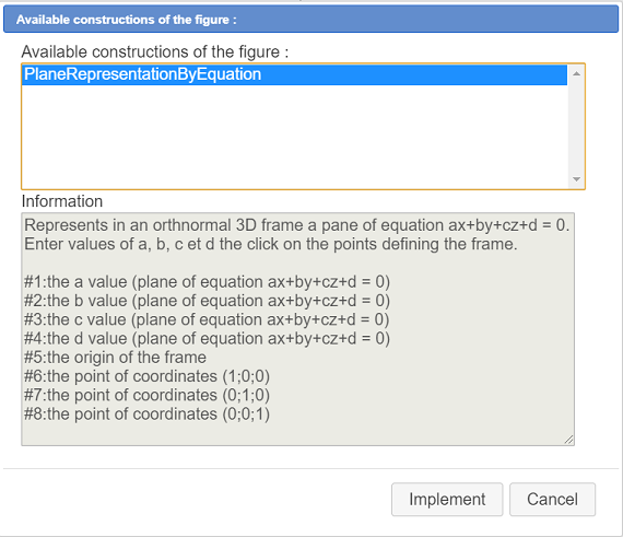
Now use icon (Macro constructions management) and choose item Incorporate a construction from a file. Browse to the directory containing the predefined constructions. Open the directory Space then the sub-directory Points and choose construction Plane representation by equation.

This construction is now part of your figure figure. To visualize this, use icon and choose item Modify the informations of a construction.

This construction needs four numerical sources objects a, b, c et d and four graphical objects that are the points defining or 3D frame : 0, I, J et K.

Again use icon and choose item Implement a construction of the figure. A dialog box pops up and our only construction is already selected. Click on button Implement.

Now we have to indicate our construction which are the sources objects.

In the left list, click on n°1. In the right list associate to source object n° 1 the calculation a (created with the first cursor) like underneath :

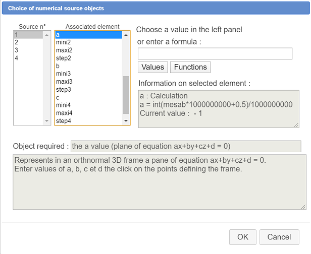
In the same way, associate to ssources objects number 2, 3 et 4 the values of b, c and d the validate. On the top right corner of the figure, a transient indicationask for you to click on the point origin of the 3D frame : click on point O. Then, in the same way, click on I, J and K.

The plane is represented by a blue parallelogram (really it is a polygon filled with a surface). Four control points allow you to get it bigger or smaller. Use icon to mask the point at the center of this parallelogram that will not be used here.

With capture tool modify the cursors to get the same values fo a, b, c and d as underneath (1, 1, 3 et 3) (lthis figure is dynamic and tou can modify values of a, b, c and d). You can also rotate the figure with $\vartheta$.

Now we will use a construction to create the orthogonal projected point of a point on a plane (and to get it’s coordinates in calculations that will be named xproj, yproj et zproj).

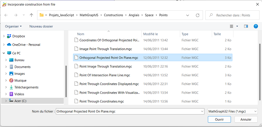
Again use icon and choose item Incorporate a construction from file, open the directory named Space then the sub-directory Points and click on the construction named Orthogonal projected point on plane. Click on button Open. like here :

This new construction is now part of our figure.

To implement it, use again icon and choose item Implement a construction of the figure.

For object source number 1 (abscissa of the point to be projected) enter directly formula 0 (abscissa of the origin) like underneath. Proceed in the samme way for sources elements n° 2 ans 3 (value 0).

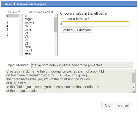
For object source n°4 we are asked for value of a : associate the already created calculation a as shown here :

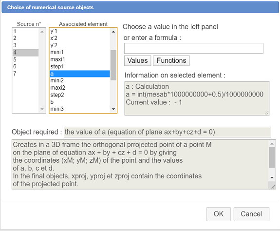
In the same way associate to sources objects numer 5, 6 and 7 the calculations b, c and d found in the list.

On the top right corner of the figure, a transient message asks you to click on the four points defining the frame : click in this order on points O, I, J and K.

A new point appears and, in the numerical objects, three calculations named xproj, yproj and zproj have been added. They contain the coordinates of this orthogonal projected point (use icon to see all the cumerical objects added to the figure). Name the new created point H with tool .

Now we will simulate a point linked to our plane. For this use icon . First click on the edge of the plane (that in fact is a polygon) then click inside the polygon. A new point appears. Name it M.

Now we will use a very powerful construction allowing us to get the coordinates of point M, knowing that M is in a plane we know an equation of

Again use icon and choose item Incorporate a construction from file, open the directory Space the the sub-directory Points and click on the construction named Computing coordinates of point in plane. Clcik on button Open.

In the dialog box popping up asign values of a, b, c et d to object sources n° 1, 2, 3 and 4.

Then you are asked to click on the point you wish to compute the coordinates : click on M. Then click on points O, I, J and K.

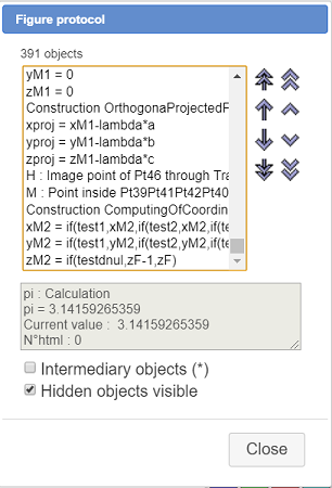
Use icon of the upper toolbar (figure protocol). Browse to the bottom of the list of created objects. The last objects created are the coordinates of point M and are named xM2, yM2 et zM2 as you can see here.

Now let us create a dynamic LaTeX display displaying the coordinates of point M.

Expand the displays toolbar and click on icon (free LaTeX display creation). Click on a free spot under the cursors.

In the dialog box popping up, enter ca M character, then click on icon . The LaTeX code display for a set of parenthesis is added : M\left( { } \right) and the caret is blinked inside the set of braces. Then click on button Value insertion. Fill in the dialog box as shown here :

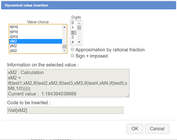
Validate. Just after add a ; character.
The LaTeX code is now : M\left( {\Val{xM2}; } \right).

Then, in the same way, use button Value insertion to insert the code for the dispaly of values xM2 et yM2 with a ; separating character.

For now our LaTeX code is :
M \left( \Val{xM2}; \Val{yM2}; \Val{zM2} \right).

We want name M not to be dispalyed in italic mode : select M in the editor the click on icon

The LaTeX code is now like underneath. Check the checkboxes Background erase et Simple frame.

\text{M} \left( \Val{xM2}; \Val{yM2}; \Val{zM2} \right)

Validate the dialog box. Our LaTeX displays appears and, if you capture point M, you see the coordinates changing in real time.

Proceed in the same way to creat a LaTeX display displaying the coordinates of point H.

The LaTeX code must be this one :
\text{H} \left( \Val{xproj}; \Val{yproj}; \Val{zproj} \right)

Now we are going to ask for the distance between O and M. For this we will use a predefined macro construction (of course we could calculate it directly).

Once more, use icon , the choose item Incorporate a construction from file and choose the file named Distance Point Point you will find in the directory Space-> Distances.

Then use again icon and choose item Implement a construction of the figure. Select in the list the last construction Distance Point Point and click on button Implement.

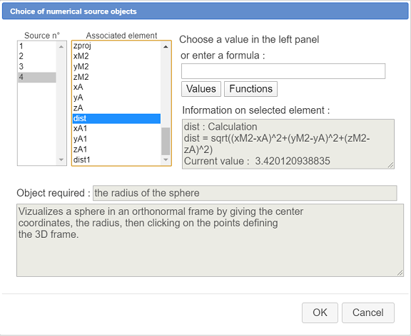
As sources objects n° 1, 2 and 3, directly enter as formula 0 in the edit field (coordinates of the origin) and assign to sources objects number 4, 5 et 6 respectivly xM2, yM2 ans zM2 (coordinates of M). A final object named dist has been created, containing the distance between O and M. You can see it with tool of the upper toolbar.

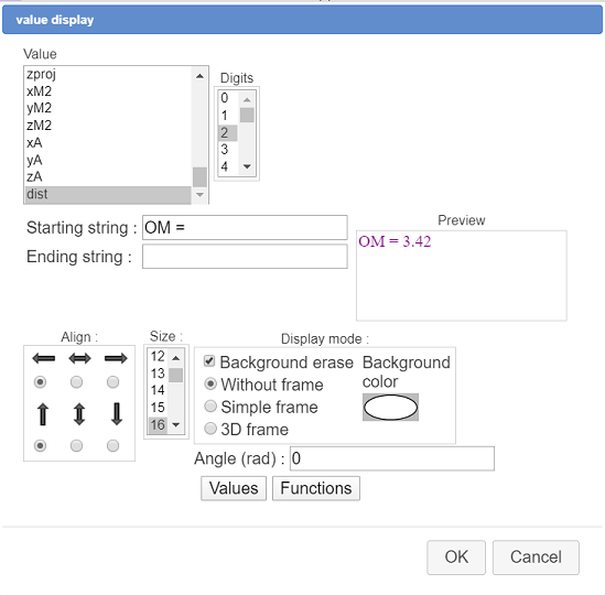
Let us now create a display of this last value. For this use icon then click under the two LaTeX displays.

Fill in the dialog box as shown here (you can use the Values button).

In the same way use the same construction to compute the distance between O and H (let us recall that H coordinates are in xproj, yproj et zproj) and create a display of this new value named (dist1) under the former display.

Our figure is now this one. Capture $\theta$ to turn the figure, capture point M or make vary the values of cursors a, b, c et d.

Now we are going to use predefined constructions to visualize the sphere of center O and going throw M and the intersection circle between this sphere and our plane.

Once again, use icon , choose item Incorporate construction from file and choose the file named Sphere Through Coord Center Radius you will find in the directory Space-> Solids.

In the same way, incorporate in the figure the construction named Circle Intersection Sphere Plane you will find in directory Line Circles.

Let us start with the sphere of center O and going through point M.

Use icon , choose item Implement a construction of the figure. Choose construction SphereThroughCoordCenterRadius and click on button Implement.

A dialog box pops up for the choice of the numerical objects. For the three first , assign the formula 0 (coordinates of O). Assign to the fourth source object the calculation dist (distance between O and M) like here.

Then you mist click on the four points defining the frame : click on O, I, J and K. The sphere representation appears (it consists of object locuses).

Now let us represent the intersection circle between the sphere and the plan.

Use icon , then choose item Implement a construction of the figure. Choose construction CircleIntersectionSpherePlane and click on button Implement.

Assign to the third sources objects the formula 0 using the edit field Formula (coordinates of the sphere center). As element associated to source n°4, click on dist. As elements associated to sources objets n°5, 6, 7 et 8 click on a, b, c et d. Validate.

Then you are asked to click on the four points defining our frame : click on O, I, J and K (for O choose free point).

A point locus appears representing the intersection.

You can change it’s line style and color using tool and fill it with tool

To finsh, activate the dotted line style, 2 pixels width, the blue color and use icon to join points O, H and M by three segments. The triangle OHM is rectangle in H and H is the center of the intersection circle.

Here is the final figure :

You can get here the Base 64 code of this figure :