Matricial calculation : Tutorial 1

Since version 6.7, MathGraph32 allows you to create and calculate matrices (with real coefficients).

In this first tutorial we will explain basic features of matricial calculation.

First create a new figure with icon of the upper toolbar. Choose a new figure witout length and without unity.

Expand the calculations toolbar (third from the bottom) and click on then right on icon (more tools).

Choose Matrix in the list. This allows you to create a matrix by choosing the numer of rows and columns ans to enter a formula for each cell of the matrix.

Fill the dialog box as below :

We are now going to ask MathGraph32 to compute the determinant of matrix A.

Once again, expand the calculations toolbar, and ckick right on icon .

Choose Determinant in the liste and validate.

A dialog box pops up.

In the list of the matrices, matrix A is already selected. Enter detA in the field Name of the calculation and validate.

If you use icon of the upper toolbar, you will see that detA value is - 6. You can use tool to display value detA on the figure.

Another way for creating a matrix is to use a matrix calculation.

Before that make sure with tool (upper toolbar) that your figure’s angle unity is the radian.

Once again use icon in the calculation expandable bar and click on Matrix calculation.

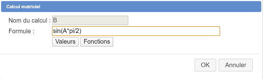
Fill in the dialog box as underneath :

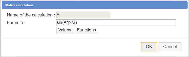
The formula for the calculation is :

sin(A*pi/2)

Now you can use tool to see the value of this matrix.

This calculation starts with multiplying each term of the matrix by pi/2 and then returns the matrix cells of which are the image of the result through sinus function.

Now we will ask for a display of this matrix B via a LaTeX display.

Click on icon (free LaTeX display), then click on the top left corner of the figure.

To enter the LaTeX code you can use the icon for inserting the parenthesis code display and the click on button Value insertion

Here is the LaTeX code :

Create a new matricial calculation named C with the formula below :

The result is the third power of matrix B (so B \times B \times B).

Please make note that the calculation of a power of a matrix is only available for a square matrix (same number of lines and columns).

Display the value of matrix C in a free LaTeX display with the LaTeX display code below :

We will use now another way of creating a matrix, giving a formula depending on i (row index starting form 1) and j (column index starting from 1.

Once again use icon in the calculation toolbar and click on Matrix by formula.

Fill in the dialog box as underneath :

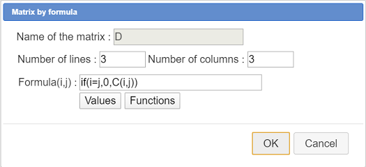
Here is the code of the formula :

So, if the row index i is equal to the column index j, the cell of the matrix will be zero (diagonla terms) and, for the other terms, the cell content will be the result of the same term in matrix C.

You can display the value of matrix C in a free LaTeX display with the LaTeX code below :

We want now to create a matrix terms of which will be the square of the terms of matrix D.

Create a new matrix by formula like this :

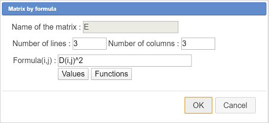
Here is the code of the formula :

You can display the value of matrix C in a free LaTeX display with the LaTeX code below :

Beware : A matricial calculation with formula D^2 will not give the same result because the result would be the product of D by D.

Create now a new matrix calculation F with formula :

This matricial product is valid because the number of columns of the first matrix D is equal to the number of rows of the second matrix E.

You can display the value of matrix C in a free LaTeX display with the LaTeX code below :

We want now to create a column matrix terms of which are the terms of the last column of matrix D.

Create a new matrix by formula G like below :

Here is the formula to be used :

You can display the value of matrix C in a free LaTeX display with the LaTeX code below :

Now create a matric calculation named H defined via this formula :

The result is a column matrix. You can display it in a free LaTeX display with the LaTeX code below :

To put an end to this tutorial, let us show that a matrix calculation can be undefined beacuse not valid.

Create a matrix calculation named J with this formula :

If you use tool of the upper toolbar you will see that this calculation is declared as non existent. Indeed, the number of columns of matrix G is not equal to the number of rows of matrix B.

So it is your responsability to make sure your matricial calculations are valid.

Here is the Base 64 code of the final figure :