Logiciel libre de géométrie, d'analyse et de simulation multiplateforme par Yves Biton
Toutes les versions de cet article : [English] [Español] [français]
In this tutorial we will create a figure where you can enter in a user-friendly way a system of 4 linear equations of 4 unknown and solve it when the solution is unique.
Her is the figure in action :
for this figure to be created, you will have to use 6.8.0 version of MathGraph32 (or a more recent version).
If you don’t want to follow all the steps of the creation, you can get here the Base 64 code of the figure :
TWF0aEdyYXBoSmF2YTEuMAAAABM+TMzNAAJmcv###wEA#wEAAAAAAAAAAAUqAAAC4AAAAQEAAAAAAAAAAQAAAEv#####AAAAAQAKQ0NhbGNDb25zdAD#####AAJwaQAWMy4xNDE1OTI2NTM1ODk3OTMyMzg0Nv####8AAAABAApDQ29uc3RhbnRlQAkh+1RELRj#####AAAAAQAJQ0ZvbmNOVmFyAP####8ABWVxdWExAAUzKng9Mf####8AAAABAApDT3BlcmF0aW9uCAAAAAMCAAAAAUAIAAAAAAAA#####wAAAAIAEUNWYXJpYWJsZUZvcm1lbGxlAAAAAAAAAAE#8AAAAAAAAAAAAAQAAXgAAXkAAXoAAXQAAAACAP####8ABWVxdWEyAAV4K3k9MgAAAAMIAAAAAwAAAAAEAAAAAAAAAAQAAAABAAAAAUAAAAAAAAAAAAAABAABeAABeQABegABdAAAAAIA#####wAFZXF1YTMAB3greSt6PTMAAAADCAAAAAMAAAAAAwAAAAAEAAAAAAAAAAQAAAABAAAABAAAAAIAAAABQAgAAAAAAAAAAAAEAAF4AAF5AAF6AAF0AAAAAgD#####AAVlcXVhNAAJeCt5K3o9NC10AAAAAwgAAAADAAAAAAMAAAAABAAAAAAAAAAEAAAAAQAAAAQAAAACAAAAAwEAAAABQBAAAAAAAAAAAAAEAAAAAwAAAAQAAXgAAXkAAXoAAXT#####AAAABAAPQ0VkaXRldXJGb3JtdWxlAP####8AAAAAAQAA#####xBAVaAAAAAAAEAxhR64UeuGAAH###8AAAACAAAAAAAAAAEAAAAAAAAAAAAAAAEADEVxdWF0aW9uIDEgOgAAABQBAQACXCwBAQAAAAUA#####wAAAAABAAD#####EEBVoAAAAAAAQE5Cj1wo9cMAAf###wAAAAIAAAAAAAAAAQAAAAAAAAAAAAAAAgAMRXF1YXRpb24gMiA6AAAAFAEBAAJcLAEBAAAABQD#####AAAAAAEAAP####8QQFUgAAAAAABAWWFHrhR64gAB####AAAAAgAAAAAAAAABAAAAAAAAAAAAAAADAAxFcXVhdGlvbiAzIDoAAAAUAQEAAlwsAQEAAAAFAP####8AAAAAAQAA#####xBAVOAAAAAAAEBicKPXCj1xAAH###8AAAACAAAAAAAAAAEAAAAAAAAAAAAAAAQADEVxdWF0aW9uIDQgOgAAABQBAQACXCwBAQAAAAIA#####wADZGYxACpsZWZ0KGVxdWExKHgseSx6LHQpKS1yaWdodChlcXVhMSh4LHkseix0KSkAAAADAf####8AAAACAAlDRm9uY3Rpb24U#####wAAAAEAEkNBcHBlbEZvbmN0aW9uTlZhcgAAAAQAAAABAAAABAAAAAAAAAAEAAAAAQAAAAQAAAACAAAABAAAAAMAAAAGFQAAAAcAAAAEAAAAAQAAAAQAAAAAAAAABAAAAAEAAAAEAAAAAgAAAAQAAAADAAAABAABeAABeQABegABdAAAAAIA#####wADZGYyACpsZWZ0KGVxdWEyKHgseSx6LHQpKS1yaWdodChlcXVhMih4LHkseix0KSkAAAADAQAAAAYUAAAABwAAAAQAAAACAAAABAAAAAAAAAAEAAAAAQAAAAQAAAACAAAABAAAAAMAAAAGFQAAAAcAAAAEAAAAAgAAAAQAAAAAAAAABAAAAAEAAAAEAAAAAgAAAAQAAAADAAAABAABeAABeQABegABdAAAAAIA#####wADZGYzACpsZWZ0KGVxdWEzKHgseSx6LHQpKS1yaWdodChlcXVhMyh4LHkseix0KSkAAAADAQAAAAYUAAAABwAAAAQAAAADAAAABAAAAAAAAAAEAAAAAQAAAAQAAAACAAAABAAAAAMAAAAGFQAAAAcAAAAEAAAAAwAAAAQAAAAAAAAABAAAAAEAAAAEAAAAAgAAAAQAAAADAAAABAABeAABeQABegABdAAAAAIA#####wADZGY0ACpsZWZ0KGVxdWE0KHgseSx6LHQpKS1yaWdodChlcXVhNCh4LHkseix0KSkAAAADAQAAAAYUAAAABwAAAAQAAAAEAAAABAAAAAAAAAAEAAAAAQAAAAQAAAACAAAABAAAAAMAAAAGFQAAAAcAAAAEAAAABAAAAAQAAAAAAAAABAAAAAEAAAAEAAAAAgAAAAQAAAADAAAABAABeAABeQABegABdP####8AAAABAAVDRm9uYwD#####AAR6ZXJvABJhYnMoeCk8MC4wMDAwMDAwMDEAAAADBAAAAAYAAAAABAAAAAAAAAABPhEuC+gm1pUAAXj#####AAAAAQARQ0Rlcml2ZWVQYXJ0aWVsbGUA#####wAFZGVyeDEAAAAJAAAAAAAAAAkA#####wAFZGVyeTEAAAAJAAAAAQAAAAkA#####wAFZGVyejEAAAAJAAAAAgAAAAkA#####wAFZGVydDEAAAAJAAAAAwAAAAkA#####wAFZGVyeDIAAAAKAAAAAAAAAAkA#####wAFZGVyeTIAAAAKAAAAAQAAAAkA#####wAFZGVyejIAAAAKAAAAAgAAAAkA#####wAFZGVydDIAAAAKAAAAAwAAAAkA#####wAFZGVyeDMAAAALAAAAAAAAAAkA#####wAFZGVyeTMAAAALAAAAAQAAAAkA#####wAFZGVyejMAAAALAAAAAgAAAAkA#####wAFZGVydDMAAAALAAAAAwAAAAkA#####wAFZGVyeDQAAAAMAAAAAAAAAAkA#####wAFZGVyeTQAAAAMAAAAAQAAAAkA#####wAFZGVyejQAAAAMAAAAAgAAAAkA#####wAFZGVydDQAAAAMAAAAA#####8AAAABAAhDTWF0cmljZQD#####AAFBAAAABAAAAAQAAAAHAAAABAAAAA4AAAABAAAAAAAAAAAAAAABAAAAAAAAAAAAAAABAAAAAAAAAAAAAAABAAAAAAAAAAAAAAAHAAAABAAAAA8AAAABAAAAAAAAAAAAAAABAAAAAAAAAAAAAAABAAAAAAAAAAAAAAABAAAAAAAAAAAAAAAHAAAABAAAABAAAAABAAAAAAAAAAAAAAABAAAAAAAAAAAAAAABAAAAAAAAAAAAAAABAAAAAAAAAAAAAAAHAAAABAAAABEAAAABAAAAAAAAAAAAAAABAAAAAAAAAAAAAAABAAAAAAAAAAAAAAABAAAAAAAAAAAAAAAHAAAABAAAABIAAAABAAAAAAAAAAAAAAABAAAAAAAAAAAAAAABAAAAAAAAAAAAAAABAAAAAAAAAAAAAAAHAAAABAAAABMAAAABAAAAAAAAAAAAAAABAAAAAAAAAAAAAAABAAAAAAAAAAAAAAABAAAAAAAAAAAAAAAHAAAABAAAABQAAAABAAAAAAAAAAAAAAABAAAAAAAAAAAAAAABAAAAAAAAAAAAAAABAAAAAAAAAAAAAAAHAAAABAAAABUAAAABAAAAAAAAAAAAAAABAAAAAAAAAAAAAAABAAAAAAAAAAAAAAABAAAAAAAAAAAAAAAHAAAABAAAABYAAAABAAAAAAAAAAAAAAABAAAAAAAAAAAAAAABAAAAAAAAAAAAAAABAAAAAAAAAAAAAAAHAAAABAAAABcAAAABAAAAAAAAAAAAAAABAAAAAAAAAAAAAAABAAAAAAAAAAAAAAABAAAAAAAAAAAAAAAHAAAABAAAABgAAAABAAAAAAAAAAAAAAABAAAAAAAAAAAAAAABAAAAAAAAAAAAAAABAAAAAAAAAAAAAAAHAAAABAAAABkAAAABAAAAAAAAAAAAAAABAAAAAAAAAAAAAAABAAAAAAAAAAAAAAABAAAAAAAAAAAAAAAHAAAABAAAABoAAAABAAAAAAAAAAAAAAABAAAAAAAAAAAAAAABAAAAAAAAAAAAAAABAAAAAAAAAAAAAAAHAAAABAAAABsAAAABAAAAAAAAAAAAAAABAAAAAAAAAAAAAAABAAAAAAAAAAAAAAABAAAAAAAAAAAAAAAHAAAABAAAABwAAAABAAAAAAAAAAAAAAABAAAAAAAAAAAAAAABAAAAAAAAAAAAAAABAAAAAAAAAAAAAAAHAAAABAAAAB0AAAABAAAAAAAAAAAAAAABAAAAAAAAAAAAAAABAAAAAAAAAAAAAAABAAAAAAAAAAD#####AAAAAQAUQ0ltcGxlbWVudGF0aW9uUHJvdG8A#####wAMRMOpdGVybWluYW50AAAAAQAAAAEAAAABAAAAHv####8AAAABAAhDQ2FsY01hdAAAAAAfAAZkZXRNYXQACGRldGVyKEEpAAAABhf#####AAAAAQAPQ1Jlc3VsdGF0VmFsZXVyAAAAHv####8AAAABAAdDQ2FsY3VsAQAAAB8ABGRldEEAC2RldE1hdCgxLDEp#####wAAAAEACENUZXJtTWF0AAAAIAAAAAE#8AAAAAAAAAAAAAE#8AAAAAAAAAAAAAoA#####wABQgAAAAQAAAAB#####wAAAAEADENNb2luc1VuYWlyZQAAAAcAAAAEAAAACQAAAAEAAAAAAAAAAAAAAAEAAAAAAAAAAAAAAAEAAAAAAAAAAAAAAAEAAAAAAAAAAAAAABAAAAAHAAAABAAAAAoAAAABAAAAAAAAAAAAAAABAAAAAAAAAAAAAAABAAAAAAAAAAAAAAABAAAAAAAAAAAAAAAQAAAABwAAAAQAAAALAAAAAQAAAAAAAAAAAAAAAQAAAAAAAAAAAAAAAQAAAAAAAAAAAAAAAQAAAAAAAAAAAAAAEAAAAAcAAAAEAAAADAAAAAEAAAAAAAAAAAAAAAEAAAAAAAAAAAAAAAEAAAAAAAAAAAAAAAEAAAAAAAAAAAAAAAwA#####wABWAAIQV4oLTEpKkIAAAADAv####8AAAABAApDUHVpc3NhbmNlAAAADQAAAB4AAAAQAAAAAT#wAAAAAAAAAAAADQAAACIAAAAOAP####8AAngwAAZYKDEsMSkAAAAPAAAAIwAAAAE#8AAAAAAAAAAAAAE#8AAAAAAAAAAAAA4A#####wACeTAABlgoMiwxKQAAAA8AAAAjAAAAAUAAAAAAAAAAAAAAAT#wAAAAAAAAAAAADgD#####AAJ6MAAGWCgzLDEpAAAADwAAACMAAAABQAgAAAAAAAAAAAABP#AAAAAAAAAAAAAOAP####8AAnQwAAZYKDQsMSkAAAAPAAAAIwAAAAFAEAAAAAAAAAAAAAE#8AAAAAAAAAAAAA4A#####wACeDEACTErcmFuZCgwKQAAAAMAAAAAAT#wAAAAAAAAAAAABhEAAAABAAAAAAAAAAA#yQx3YPYD6AAAAA4A#####wACeDIACTErcmFuZCgwKQAAAAMAAAAAAT#wAAAAAAAAAAAABhEAAAABAAAAAAAAAAA#xwLfiiKFAAAAAA4A#####wACeDMACTErcmFuZCgwKQAAAAMAAAAAAT#wAAAAAAAAAAAABhEAAAABAAAAAAAAAAA#3k0M#OgOPAAAAA4A#####wACeTEACzEuMStyYW5kKDApAAAAAwAAAAABP#GZmZmZmZoAAAAGEQAAAAEAAAAAAAAAAD#v4UKKWPSGAAAADgD#####AAJ5MgALMS4xK3JhbmQoMCkAAAADAAAAAAE#8ZmZmZmZmgAAAAYRAAAAAQAAAAAAAAAAP+SfTcsseUAAAAAOAP####8AAnkzAAsxLjErcmFuZCgwKQAAAAMAAAAAAT#xmZmZmZmaAAAABhEAAAABAAAAAAAAAAA#0b7YIwpBfAAAAA4A#####wACejEACzEuMityYW5kKDApAAAAAwAAAAABP#MzMzMzMzMAAAAGEQAAAAEAAAAAAAAAAD#o+Ys1fE7YAAAADgD#####AAJ6MgALMS4yK3JhbmQoMCkAAAADAAAAAAE#8zMzMzMzMwAAAAYRAAAAAQAAAAAAAAAAP+44hIFCCa4AAAAOAP####8AAnozAAsxLjIrcmFuZCgwKQAAAAMAAAAAAT#zMzMzMzMzAAAABhEAAAABAAAAAAAAAAA#6lahQDQ#vAAAAA4A#####wACdDEACzEuMytyYW5kKDApAAAAAwAAAAABP#TMzMzMzM0AAAAGEQAAAAEAAAAAAAAAAD+6PypCjAyAAAAADgD#####AAJ0MgALMS4zK3JhbmQoMCkAAAADAAAAAAE#9MzMzMzMzQAAAAYRAAAAAQAAAAAAAAAAP9ZrtjYzU3wAAAAOAP####8AAnQzAAsxLjMrcmFuZCgwKQAAAAMAAAAAAT#0zMzMzMzNAAAABhEAAAABAAAAAAAAAAA#sMtc7DidUAAAAA4A#####wAEZGVnMQFfemVybyhkZXJ4MSh4MSx5MSx6MSx0MSktZGVyeDEoeDIseTIsejIsdDIpKSZ6ZXJvKGRlcngxKHgyLHkyLHoyLHQyKS1kZXJ4MSh4Myx5Myx6Myx0MykpJnplcm8oZGVyeTEoeDEseTEsejEsdDEpLWRlcnkxKHgyLHkyLHoyLHQyKSkmemVybyhkZXJ5MSh4Mix5Mix6Mix0MiktZGVyeTEoeDMseTMsejMsdDMpKSZ6ZXJvKGRlcnoxKHgxLHkxLHoxLHQxKS1kZXJ6MSh4Mix5Mix6Mix0MikpJnplcm8oZGVyejEoeDIseTIsejIsdDIpLWRlcnoxKHgzLHkzLHozLHQzKSkmemVybyhkZXJ0MSh4MSx5MSx6MSx0MSktZGVydDEoeDIseTIsejIsdDIpKSZ6ZXJvKGRlcnQxKHgyLHkyLHoyLHQyKS1kZXJ0MSh4Myx5Myx6Myx0MykpAAAAAwoAAAADCgAAAAMKAAAAAwoAAAADCgAAAAMKAAAAAwr#####AAAAAQAOQ0FwcGVsRm9uY3Rpb24AAAANAAAAAwEAAAAHAAAABAAAAA4AAAANAAAAKAAAAA0AAAArAAAADQAAAC4AAAANAAAAMQAAAAcAAAAEAAAADgAAAA0AAAApAAAADQAAACwAAAANAAAALwAAAA0AAAAyAAAAEgAAAA0AAAADAQAAAAcAAAAEAAAADgAAAA0AAAApAAAADQAAACwAAAANAAAALwAAAA0AAAAyAAAABwAAAAQAAAAOAAAADQAAACoAAAANAAAALQAAAA0AAAAwAAAADQAAADMAAAASAAAADQAAAAMBAAAABwAAAAQAAAAPAAAADQAAACgAAAANAAAAKwAAAA0AAAAuAAAADQAAADEAAAAHAAAABAAAAA8AAAANAAAAKQAAAA0AAAAsAAAADQAAAC8AAAANAAAAMgAAABIAAAANAAAAAwEAAAAHAAAABAAAAA8AAAANAAAAKQAAAA0AAAAsAAAADQAAAC8AAAANAAAAMgAAAAcAAAAEAAAADwAAAA0AAAAqAAAADQAAAC0AAAANAAAAMAAAAA0AAAAzAAAAEgAAAA0AAAADAQAAAAcAAAAEAAAAEAAAAA0AAAAoAAAADQAAACsAAAANAAAALgAAAA0AAAAxAAAABwAAAAQAAAAQAAAADQAAACkAAAANAAAALAAAAA0AAAAvAAAADQAAADIAAAASAAAADQAAAAMBAAAABwAAAAQAAAAQAAAADQAAACkAAAANAAAALAAAAA0AAAAvAAAADQAAADIAAAAHAAAABAAAABAAAAANAAAAKgAAAA0AAAAtAAAADQAAADAAAAANAAAAMwAAABIAAAANAAAAAwEAAAAHAAAABAAAABEAAAANAAAAKAAAAA0AAAArAAAADQAAAC4AAAANAAAAMQAAAAcAAAAEAAAAEQAAAA0AAAApAAAADQAAACwAAAANAAAALwAAAA0AAAAyAAAAEgAAAA0AAAADAQAAAAcAAAAEAAAAEQAAAA0AAAApAAAADQAAACwAAAANAAAALwAAAA0AAAAyAAAABwAAAAQAAAARAAAADQAAACoAAAANAAAALQAAAA0AAAAwAAAADQAAADMAAAAOAP####8ABGRlZzIBX3plcm8oZGVyeDIoeDEseTEsejEsdDEpLWRlcngyKHgyLHkyLHoyLHQyKSkmemVybyhkZXJ4Mih4Mix5Mix6Mix0MiktZGVyeDIoeDMseTMsejMsdDMpKSZ6ZXJvKGRlcnkyKHgxLHkxLHoxLHQxKS1kZXJ5Mih4Mix5Mix6Mix0MikpJnplcm8oZGVyeTIoeDIseTIsejIsdDIpLWRlcnkyKHgzLHkzLHozLHQzKSkmemVybyhkZXJ6Mih4MSx5MSx6MSx0MSktZGVyejIoeDIseTIsejIsdDIpKSZ6ZXJvKGRlcnoyKHgyLHkyLHoyLHQyKS1kZXJ6Mih4Myx5Myx6Myx0MykpJnplcm8oZGVydDIoeDEseTEsejEsdDEpLWRlcnQyKHgyLHkyLHoyLHQyKSkmemVybyhkZXJ0Mih4Mix5Mix6Mix0MiktZGVydDIoeDMseTMsejMsdDMpKQAAAAMKAAAAAwoAAAADCgAAAAMKAAAAAwoAAAADCgAAAAMKAAAAEgAAAA0AAAADAQAAAAcAAAAEAAAAEgAAAA0AAAAoAAAADQAAACsAAAANAAAALgAAAA0AAAAxAAAABwAAAAQAAAASAAAADQAAACkAAAANAAAALAAAAA0AAAAvAAAADQAAADIAAAASAAAADQAAAAMBAAAABwAAAAQAAAASAAAADQAAACkAAAANAAAALAAAAA0AAAAvAAAADQAAADIAAAAHAAAABAAAABIAAAANAAAAKgAAAA0AAAAtAAAADQAAADAAAAANAAAAMwAAABIAAAANAAAAAwEAAAAHAAAABAAAABMAAAANAAAAKAAAAA0AAAArAAAADQAAAC4AAAANAAAAMQAAAAcAAAAEAAAAEwAAAA0AAAApAAAADQAAACwAAAANAAAALwAAAA0AAAAyAAAAEgAAAA0AAAADAQAAAAcAAAAEAAAAEwAAAA0AAAApAAAADQAAACwAAAANAAAALwAAAA0AAAAyAAAABwAAAAQAAAATAAAADQAAACoAAAANAAAALQAAAA0AAAAwAAAADQAAADMAAAASAAAADQAAAAMBAAAABwAAAAQAAAAUAAAADQAAACgAAAANAAAAKwAAAA0AAAAuAAAADQAAADEAAAAHAAAABAAAABQAAAANAAAAKQAAAA0AAAAsAAAADQAAAC8AAAANAAAAMgAAABIAAAANAAAAAwEAAAAHAAAABAAAABQAAAANAAAAKQAAAA0AAAAsAAAADQAAAC8AAAANAAAAMgAAAAcAAAAEAAAAFAAAAA0AAAAqAAAADQAAAC0AAAANAAAAMAAAAA0AAAAzAAAAEgAAAA0AAAADAQAAAAcAAAAEAAAAFQAAAA0AAAAoAAAADQAAACsAAAANAAAALgAAAA0AAAAxAAAABwAAAAQAAAAVAAAADQAAACkAAAANAAAALAAAAA0AAAAvAAAADQAAADIAAAASAAAADQAAAAMBAAAABwAAAAQAAAAVAAAADQAAACkAAAANAAAALAAAAA0AAAAvAAAADQAAADIAAAAHAAAABAAAABUAAAANAAAAKgAAAA0AAAAtAAAADQAAADAAAAANAAAAMwAAAA4A#####wAEZGVnMwFfemVybyhkZXJ4Myh4MSx5MSx6MSx0MSktZGVyeDMoeDIseTIsejIsdDIpKSZ6ZXJvKGRlcngzKHgyLHkyLHoyLHQyKS1kZXJ4Myh4Myx5Myx6Myx0MykpJnplcm8oZGVyeTMoeDEseTEsejEsdDEpLWRlcnkzKHgyLHkyLHoyLHQyKSkmemVybyhkZXJ5Myh4Mix5Mix6Mix0MiktZGVyeTMoeDMseTMsejMsdDMpKSZ6ZXJvKGRlcnozKHgxLHkxLHoxLHQxKS1kZXJ6Myh4Mix5Mix6Mix0MikpJnplcm8oZGVyejMoeDIseTIsejIsdDIpLWRlcnozKHgzLHkzLHozLHQzKSkmemVybyhkZXJ0Myh4MSx5MSx6MSx0MSktZGVydDMoeDIseTIsejIsdDIpKSZ6ZXJvKGRlcnQzKHgyLHkyLHoyLHQyKS1kZXJ0Myh4Myx5Myx6Myx0MykpAAAAAwoAAAADCgAAAAMKAAAAAwoAAAADCgAAAAMKAAAAAwoAAAASAAAADQAAAAMBAAAABwAAAAQAAAAWAAAADQAAACgAAAANAAAAKwAAAA0AAAAuAAAADQAAADEAAAAHAAAABAAAABYAAAANAAAAKQAAAA0AAAAsAAAADQAAAC8AAAANAAAAMgAAABIAAAANAAAAAwEAAAAHAAAABAAAABYAAAANAAAAKQAAAA0AAAAsAAAADQAAAC8AAAANAAAAMgAAAAcAAAAEAAAAFgAAAA0AAAAqAAAADQAAAC0AAAANAAAAMAAAAA0AAAAzAAAAEgAAAA0AAAADAQAAAAcAAAAEAAAAFwAAAA0AAAAoAAAADQAAACsAAAANAAAALgAAAA0AAAAxAAAABwAAAAQAAAAXAAAADQAAACkAAAANAAAALAAAAA0AAAAvAAAADQAAADIAAAASAAAADQAAAAMBAAAABwAAAAQAAAAXAAAADQAAACkAAAANAAAALAAAAA0AAAAvAAAADQAAADIAAAAHAAAABAAAABcAAAANAAAAKgAAAA0AAAAtAAAADQAAADAAAAANAAAAMwAAABIAAAANAAAAAwEAAAAHAAAABAAAABgAAAANAAAAKAAAAA0AAAArAAAADQAAAC4AAAANAAAAMQAAAAcAAAAEAAAAGAAAAA0AAAApAAAADQAAACwAAAANAAAALwAAAA0AAAAyAAAAEgAAAA0AAAADAQAAAAcAAAAEAAAAGAAAAA0AAAApAAAADQAAACwAAAANAAAALwAAAA0AAAAyAAAABwAAAAQAAAAYAAAADQAAACoAAAANAAAALQAAAA0AAAAwAAAADQAAADMAAAASAAAADQAAAAMBAAAABwAAAAQAAAAZAAAADQAAACgAAAANAAAAKwAAAA0AAAAuAAAADQAAADEAAAAHAAAABAAAABkAAAANAAAAKQAAAA0AAAAsAAAADQAAAC8AAAANAAAAMgAAABIAAAANAAAAAwEAAAAHAAAABAAAABkAAAANAAAAKQAAAA0AAAAsAAAADQAAAC8AAAANAAAAMgAAAAcAAAAEAAAAGQAAAA0AAAAqAAAADQAAAC0AAAANAAAAMAAAAA0AAAAzAAAADgD#####AARkZWc0AV96ZXJvKGRlcng0KHgxLHkxLHoxLHQxKS1kZXJ4NCh4Mix5Mix6Mix0MikpJnplcm8oZGVyeDQoeDIseTIsejIsdDIpLWRlcng0KHgzLHkzLHozLHQzKSkmemVybyhkZXJ5NCh4MSx5MSx6MSx0MSktZGVyeTQoeDIseTIsejIsdDIpKSZ6ZXJvKGRlcnk0KHgyLHkyLHoyLHQyKS1kZXJ5NCh4Myx5Myx6Myx0MykpJnplcm8oZGVyejQoeDEseTEsejEsdDEpLWRlcno0KHgyLHkyLHoyLHQyKSkmemVybyhkZXJ6NCh4Mix5Mix6Mix0MiktZGVyejQoeDMseTMsejMsdDMpKSZ6ZXJvKGRlcnQ0KHgxLHkxLHoxLHQxKS1kZXJ0NCh4Mix5Mix6Mix0MikpJnplcm8oZGVydDQoeDIseTIsejIsdDIpLWRlcnQ0KHgzLHkzLHozLHQzKSkAAAADCgAAAAMKAAAAAwoAAAADCgAAAAMKAAAAAwoAAAADCgAAABIAAAANAAAAAwEAAAAHAAAABAAAABoAAAANAAAAKAAAAA0AAAArAAAADQAAAC4AAAANAAAAMQAAAAcAAAAEAAAAGgAAAA0AAAApAAAADQAAACwAAAANAAAALwAAAA0AAAAyAAAAEgAAAA0AAAADAQAAAAcAAAAEAAAAGgAAAA0AAAApAAAADQAAACwAAAANAAAALwAAAA0AAAAyAAAABwAAAAQAAAAaAAAADQAAACoAAAANAAAALQAAAA0AAAAwAAAADQAAADMAAAASAAAADQAAAAMBAAAABwAAAAQAAAAbAAAADQAAACgAAAANAAAAKwAAAA0AAAAuAAAADQAAADEAAAAHAAAABAAAABsAAAANAAAAKQAAAA0AAAAsAAAADQAAAC8AAAANAAAAMgAAABIAAAANAAAAAwEAAAAHAAAABAAAABsAAAANAAAAKQAAAA0AAAAsAAAADQAAAC8AAAANAAAAMgAAAAcAAAAEAAAAGwAAAA0AAAAqAAAADQAAAC0AAAANAAAAMAAAAA0AAAAzAAAAEgAAAA0AAAADAQAAAAcAAAAEAAAAHAAAAA0AAAAoAAAADQAAACsAAAANAAAALgAAAA0AAAAxAAAABwAAAAQAAAAcAAAADQAAACkAAAANAAAALAAAAA0AAAAvAAAADQAAADIAAAASAAAADQAAAAMBAAAABwAAAAQAAAAcAAAADQAAACkAAAANAAAALAAAAA0AAAAvAAAADQAAADIAAAAHAAAABAAAABwAAAANAAAAKgAAAA0AAAAtAAAADQAAADAAAAANAAAAMwAAABIAAAANAAAAAwEAAAAHAAAABAAAAB0AAAANAAAAKAAAAA0AAAArAAAADQAAAC4AAAANAAAAMQAAAAcAAAAEAAAAHQAAAA0AAAApAAAADQAAACwAAAANAAAALwAAAA0AAAAyAAAAEgAAAA0AAAADAQAAAAcAAAAEAAAAHQAAAA0AAAApAAAADQAAACwAAAANAAAALwAAAA0AAAAyAAAABwAAAAQAAAAdAAAADQAAACoAAAANAAAALQAAAA0AAAAwAAAADQAAADMAAAACAP####8ABGVnYWwAA3g9MAAAAAMIAAAABAAAAAAAAAABAAAAAAAAAAAAAAAEAAF4AAF5AAF6AAF0#####wAAAAEADENUZXN0RXFOYXRPcAD#####AAdlZ2FsZXExAAAAAQAAADgAAAATAP####8AB2VnYWxlcTIAAAABAAAAOAAAABMA#####wAHZWdhbGVxMwAAAAEAAAA4AAAAEwD#####AAdlZ2FsZXE0AAAABAAAADgAAAAMAP####8AB3NvbGZyYWMAB2ZyYWMoWCkAAAAGGQAAAA0AAAAjAAAADgD#####AANueDAADHNvbGZyYWMoMSwxKQAAAA8AAAA9AAAAAT#wAAAAAAAAAAAAAT#wAAAAAAAAAAAADgD#####AANkeDAADHNvbGZyYWMoMSwyKQAAAA8AAAA9AAAAAT#wAAAAAAAAAAAAAUAAAAAAAAAAAAAADgD#####AANueTAADHNvbGZyYWMoMiwxKQAAAA8AAAA9AAAAAUAAAAAAAAAAAAAAAT#wAAAAAAAAAAAADgD#####AANkeTAADHNvbGZyYWMoMiwyKQAAAA8AAAA9AAAAAUAAAAAAAAAAAAAAAUAAAAAAAAAAAAAADgD#####AANuejAADHNvbGZyYWMoMywxKQAAAA8AAAA9AAAAAUAIAAAAAAAAAAAAAT#wAAAAAAAAAAAADgD#####AANkejAADHNvbGZyYWMoMywyKQAAAA8AAAA9AAAAAUAIAAAAAAAAAAAAAUAAAAAAAAAAAAAADgD#####AANudDAADHNvbGZyYWMoNCwxKQAAAA8AAAA9AAAAAUAQAAAAAAAAAAAAAT#wAAAAAAAAAAAADgD#####AANkdDAADHNvbGZyYWMoNCwyKQAAAA8AAAA9AAAAAUAQAAAAAAAAAAAAAUAAAAAAAAAAAAAADgD#####AAdjb3JyZWN0ADNkZWcxJmRlZzImZGVnMyZkZWc0JmVnYWxlcTEmZWdhbGVxMiZlZ2FsZXEzJmVnYWxlcTQAAAADCgAAAAMKAAAAAwoAAAADCgAAAAMKAAAAAwoAAAADCgAAAA0AAAA0AAAADQAAADUAAAANAAAANgAAAA0AAAA3AAAADQAAADkAAAANAAAAOgAAAA0AAAA7AAAADQAAADwAAAAOAP####8ABm9uZXNvbAAHZGV0QTw+MAAAAAMJAAAADQAAACEAAAABAAAAAAAAAAAAAAAIAP####8ABnplcm8xNAAPYWJzKHgpPDEwXigtMTQpAAAAAwQAAAAGAAAAAAQAAAAAAAAAEQAAAAFAJAAAAAAAAAAAABAAAAABQCwAAAAAAAAAAXgAAAAOAP####8ABWV4YWN0AEt6ZXJvMTQobngwL2R4MC14MCkmemVybzE0KG55MC9keTAteTApJnplcm8xNChuejAvZHowLXowKSZ6ZXJvMTQobnQwL2R0MC10MCkAAAADCgAAAAMKAAAAAwoAAAASAAAASAAAAAMBAAAAAwMAAAANAAAAPgAAAA0AAAA#AAAADQAAACQAAAASAAAASAAAAAMBAAAAAwMAAAANAAAAQAAAAA0AAABBAAAADQAAACUAAAASAAAASAAAAAMBAAAAAwMAAAANAAAAQgAAAA0AAABDAAAADQAAACYAAAASAAAASAAAAAMBAAAAAwMAAAANAAAARAAAAA0AAABFAAAADQAAACf#####AAAAAgAGQ0xhdGV4AP####8AAAD#AQAA#####xNAHgAAAAAAAEBrEKPXCj1xAQHv7#sAAAAAAAAAAAAAAAEAAAAAAAAAAAIPXElme2NvcnJlY3R9CnsKXElme29uZXNvbH0KewpcYmVnaW57YXJyYXl9e2x9Clx0ZXh0e1RoZSBzeXN0ZW0gaGFzIGFuIHVuaXF1ZSBzb2x1dGlvbiAoJHgkOyR5JDskeiQsJHQkKSBzb2x1dGlvbiB9IApcXCBcbGVmdCggXGJlZ2lue2FycmF5fXtsfSB4IFxcIHlcXCB6IFxcIHQgXGVuZHthcnJheX0gXHJpZ2h0KVxhcHByb3ggXGxlZnQoIFxWYWx7WCwxMn0gXHJpZ2h0KQpcXCBcdGV4dHtSYXRpb25hbCBzb2x1dGlvbiBcSWZ7ZXhhY3R9e317YXBwcm94aW1hdGVkIDogfX0KXGxlZnQoIFxiZWdpbnthcnJheX17bH0geCBcXCB5XFwgeiBcXCB0IFxlbmR7YXJyYXl9IFxyaWdodCkgXElmIHtleGFjdH17PX17XGFwcHJveH0gXGxlZnQoIFxWYWxGcmFje1h9IFxyaWdodCkKXGVuZHthcnJheX0KfQp7Clx0ZXh0Y29sb3J7cmVkfXtcdGV4dHtUaGUgc3lzdGVtIGhhcyBub3QgYW4gdW5pcXVlIHNvbHV0aW9ufX0KfQoKfQp7Clx0ZXh0Y29sb3J7cmVkfXtcdGV4dHtTeXN0w6htZSBpbmNvcnJlY3Qgb3Ugbm9uIGxpbsOpYWlyZX19Cn3###############8=Start up MathGraph32 (6.8.0 or more recent) and use icon  to create a new figure without frame and without unity length.
The four equations will be contained in four functions of four variables (feature only available since 6.8.0 version).
Expand the calculation toolbar and click on the right on icon  . Choose Real function of three variables or more.
A dialog box pops up. Fill it in as shown above :
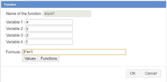
Proceed in the same way to create three other functions of variables x, y, z et t with the formulas underneath :
| Function name | Formula |
| equa2 | x+y=2 |
| equa3 | x+y+z=3 |
| equa4 | x+y+z=4-t |
Later we will be able to modify these equations but for now we know that our system has an unique solution $(x ;y ;z ;t)=(1 ;1 ;1 ;1)$
Now let’s associate to these four functions four formula editors. These editors will allow us to modify the four equations of the system to be solved.
Expand the display toolbar and click on icon  .
.
Click on the top left corner of the figure and fill in the dialog box as shown underneath :
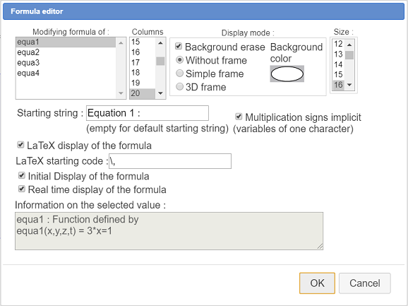
Proceed in the same way to create three formula editors associated with functions equa2, equa3, equa4 and align them with the first one. To move a formula editor, capture it with tool  (the active area for capture is the starting string).
Again, create four functions of variables x, y, z et t with the formulas abobe :
| Functio name | Formula |
| df1 | left(equa1(x,y,z,t))-right(equa1(x,y,z,t)) |
| df2 | left(equa2(x,y,z,t))-right(equa2(x,y,z,t)) |
| df3 | left(equa3(x,y,z,t))-right(equa3(x,y,z,t)) |
| df4 | left(equa4(x,y,z,t))-right(equa4(x,y,z,t)) |
Operators left and right extract the left or right part of the top calculations’s operator (here an equality).
Again, expand the calculations toolbar, click on icon and choose Partial derivative.
The first partial derivative to be created is the derivative of function equa1 relative to variable x as underneath.
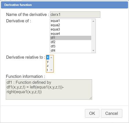
Here are the 16 partial derivatives to be created :
| Nom de la dérivée partielle | Dérivée de | Variable de dérivation |
| derx1 | df1 | x |
| dery1 | df1 | y |
| derz1 | df1 | z |
| dert1 | df1 | t |
| derx2 | df2 | x |
| dery2 | df2 | y |
| derz2 | df2 | z |
| dert2 | df2 | t |
| derx3 | df3 | x |
| dery3 | df3 | y |
| derz3 | df3 | z |
| dert3 | df3 | t |
| derx4 | df4 | x |
| dery4 | df4 | y |
| derz4 | df4 | z |
| dert4 | df4 | t |
We will now create a matrix A of four rows and four columns.
For this, expand again the calculations toolbar, click on icon and choose Matrix.
Fill in the dialog box as shown here :
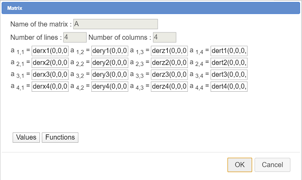
The first formula is for instance : derx1(0,0,0,0) (since derx1 is a function of four variables being partial derivative of a four variable function).
Here are the 16 formulas for the 16 matrix cells formules pour les 16 éléments de la matrice :
| Elément | Formule |
| $a_{11}$ | derx1(0,0,0,0) |
| $a_{12}$ | dery1(0,0,0,0) |
| $a_{13}$ | derz1(0,0,0,0) |
| $a_{14}$ | dert1(0,0,0,0) |
| $a_{21}$ | derx2(0,0,0,0) |
| $a_{22}$ | dery2(0,0,0,0) |
| $a_{23}$ | derz2(0,0,0,0) |
| $a_{24}$ | dert2(0,0,0,0) |
| $a_{31}$ | derx3(0,0,0,0) |
| $a_{32}$ | dery3(0,0,0,0) |
| $a_{33}$ | derz3(0,0,0,0) |
| $a_{34}$ | dert3(0,0,0,0) |
| $a_{41}$ | derx4(0,0,0,0) |
| $a_{42}$ | dery4(0,0,0,0) |
| $a_{43}$ | derz4(0,0,0,0) |
| $a_{44}$ | dert4(0,0,0,0) |
Proceed in the same way to create a real matrix B of three rows and one column as shown here :
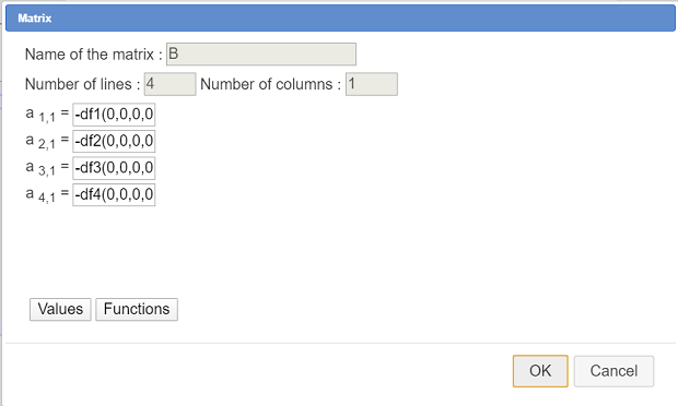
Here are the formulas for the four matrix cells :
| Elément | Formule |
| $b_{11}$ | -df1(0,0,0,0) |
| $b_{21}$ | -df2(0,0,0,0) |
| $b_{31}$ | -df3(0,0,0,0) |
| $b_{41}$ | -d4(0,0,0,0) |
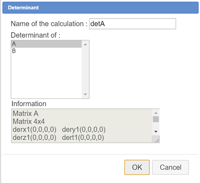
We are now going to create matrix A determinant. This determinant will indicate whether the system has an unique solution or not.
Expand again the calculations toolbar, click on icon and choose Determinant.
Fill in the dialog box as indicated below :
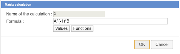
Let us cfreate now a matrix calculation named X which will contain the solution of the system (when the solution is unique).
Expand the calculations toolbar, click on icon and choose Matricial calculation.
Fill in the dialog box as underneath :
Now use icon  to create the following calculations :
| Calculation name | Formula | Explanation |
| x0 | X(1,1) | Contains x value of the solution if unique |
| y0 | X(2,1) | Contains y value of the solution if unique |
| z0 | X(3,1) | Contains z value of the solution if unique |
| t0 | X(4,1) | Contains t value of the solution if unique |
| x1 | 1+rand(0) | Random value used to verify that the partial derivatives are constant |
| x2 | 1+rand(0) | |
| x3 | 1+rand(0) | |
| y1 | 1.1+rand(0) | |
| y2 | 1.1+rand(0) | |
| y3 | 1.1+rand(0) | |
| z1 | 1.2+rand(0) | |
| z2 | 1.2+rand(0) | |
| z3 | 1.2+rand(0) | |
| t1 | 1.3+rand(0) | |
| t2 | 1.3+rand(0) | |
| t3 | 1.3+rand(0) |
Now create four real calculations named deg1, deg2, deg3 and deg4 with the following formulas :
For deg1 :
zero(derx1(x1,y1,z1,t1)-derx1(x2,y2,z2,t2))&zero(derx1(x2,y2,z2,t2)-derx1(x3,y3,z3,t3))&zero(dery1(x1,y1,z1,t1)-dery1(x2,y2,z2,t2))&zero(dery1(x2,y2,z2,t2)-dery1(x3,y3,z3,t3))&zero(derz1(x1,y1,z1,t1)-derz1(x2,y2,z2,t2))&zero(derz1(x2,y2,z2,t2)-derz1(x3,y3,z3,t3))&zero(dert1(x1,y1,z1,t1)-dert1(x2,y2,z2,t2))&zero(dert1(x2,y2,z2,t2)-dert1(x3,y3,z3,t3))For deg2 :
zero(derx2(x1,y1,z1,t1)-derx2(x2,y2,z2,t2))&zero(derx2(x2,y2,z2,t2)-derx2(x3,y3,z3,t3))&zero(dery2(x1,y1,z1,t1)-dery2(x2,y2,z2,t2))&zero(dery2(x2,y2,z2,t2)-dery2(x3,y3,z3,t3))&zero(derz2(x1,y1,z1,t1)-derz2(x2,y2,z2,t2))&zero(derz2(x2,y2,z2,t2)-derz2(x3,y3,z3,t3))&zero(dert2(x1,y1,z1,t1)-dert2(x2,y2,z2,t2))&zero(dert2(x2,y2,z2,t2)-dert2(x3,y3,z3,t3))For deg3 :
zero(derx3(x1,y1,z1,t1)-derx3(x2,y2,z2,t2))&zero(derx3(x2,y2,z2,t2)-derx3(x3,y3,z3,t3))&zero(dery3(x1,y1,z1,t1)-dery3(x2,y2,z2,t2))&zero(dery3(x2,y2,z2,t2)-dery3(x3,y3,z3,t3))&zero(derz3(x1,y1,z1,t1)-derz3(x2,y2,z2,t2))&zero(derz3(x2,y2,z2,t2)-derz3(x3,y3,z3,t3))&zero(dert3(x1,y1,z1,t1)-dert3(x2,y2,z2,t2))&zero(dert3(x2,y2,z2,t2)-dert3(x3,y3,z3,t3))For deg4 :
zero(derx4(x1,y1,z1,t1)-derx4(x2,y2,z2,t2))&zero(derx4(x2,y2,z2,t2)-derx4(x3,y3,z3,t3))&zero(dery4(x1,y1,z1,t1)-dery4(x2,y2,z2,t2))&zero(dery4(x2,y2,z2,t2)-dery4(x3,y3,z3,t3))&zero(derz4(x1,y1,z1,t1)-derz4(x2,y2,z2,t2))&zero(derz4(x2,y2,z2,t2)-derz4(x3,y3,z3,t3))&zero(dert4(x1,y1,z1,t1)-dert4(x2,y2,z2,t2))&zero(dert4(x2,y2,z2,t2)-dert4(x3,y3,z3,t3))For instance, deg1 value will be 1 if the equation contained in equa1 is of first degree relatively to variables x, y, z et t.
We also have to check if the formulas contained in functions equa1, equa2, equa3 et equa4 are equalities.
For this we will create a real function of four variables with an equality as formula.
So let us create a real function of 4 variables named egal with formula x=0 (any formula will be OK if it is an equality).
Expand the calculations toolbar, click on icon and choose Operator nature test.
Create the first test named egaleq1 like underneath :
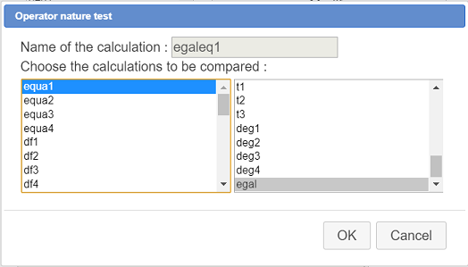
Then create three other nature operator tests :
| Name of the operator nature test | Test between |
| egaleq2 | equa2 and egal |
| egaleq3 | equa3 and egal |
| egaleq4 | equa4 and egal |
Now we are going to create approximated rational values for the x, y, z and t values of the solution (if unique).
For this we will use a matricial calculation.
Since the introduction of matricial calculation, a new function frac has been added and can be used in real calculations.
frac can be applied to a real number, a matrix of one column or a matrix of one row.
Applied to a column matrix of n rows, frac returns a matrix of n rows and two columns. The first column of the result contains the numerators of the approximated rational values of the initial matrix (rounded to 10^-12 ) and the second column constains the denominators.
Expand the calculations toolbar, click on icon and choose Matricial calculation.
Create a matrix calculation named solfrac as shown here :
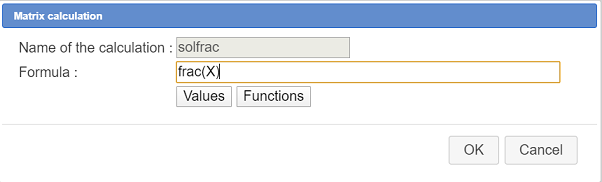
The formula to be used is : frac(X)
Now we are going to get the numerators and denominators of the rational approximated solutions in real calculations.
Create the following real calculations (icon ) :
| Calculation name | Formula |
| nx0 | solfrac(1,1) |
| dx0 | solfrac(1,2) |
| ny0 | solfrac(2,1) |
| dx0 | solfrac(2,2) |
| nz0 | solfrac(3,1) |
| dz0 | solfrac(3,2) |
| nt0 | solfrac(4,1) |
| dt0 | solfrac(4,2) |
| correct | deg1°2°3°4&egaleq1&egaleq2&egaleq3&egaleq4 |
The last calculation correct will return value 1 if the system is linear and has equalities in each equation and 0 otherwise.
Use icon to create a real calculation named onesol with the following formula :
detA<>0
onesol value will be 1 if the system has an unique solution, 0 otherwise.
Now use icon  to create a real function of variable x named zero14 with the following formula :
abs(x)<10^(-14)
Our rational approximation through frac function is rounded to 10^(-12).
If the distance between the rational approximations and the solutions contained in (x0, y0, z0, t0) is less than 10^(-14) we will consider our rational approximations as an exact solution.
Use icon to create a real calculation named
exact with the following formula :
zero14(nx0/dx0-x0)&zero14(ny0/dy0-y0)&zero14(nz0/dz0-z0)&zero14(nt0/dt0-t0)All we have to do now is create a LaTeX display displaying the solution when the solution is unique, or a warning if the system is non linear or if the solution is not unique.
in the display toolbar, use icon  .
.
Click under the formula editors to indicate the spot the LaTeX is to be displayed at.
Use the following LaTeX code :
This LaTeX display uses conditional \If functions (specific to MathGraph32).
The syntax is \If{condition} {LaTeX code if condition equals 1}{LaTeX code otherwise}
LaTeX code \Val{X,12} gets the display of matrix X, each term rounded to 12 decimal places.
LaTeX code \ValFrac{X} gets the display of matrix X where each term is represented as an approximated rational value rounded at 10^(-12) .
You can now modify the formula editors to solve the system of tour choice.
For instance, if you set the first equation to x²=1, the system will be declared as non linear.
If you set the first equation to 3x = 1without changing the last three ones you will see that the rational solution (1/3 ; 5/3 ; 1 ; 1) is declared as exact.
But if you set the first equation to 3x=1.0000000000001the same rational solution is declared as approximated.
 Accueil
 Présentation
 FAQ
FAQ Contact